[TS] HW02

해당 자료는 전북대학교 이영미 교수님 2023고급시계열분석 자료임

getwd()

setwd("/home/coco/Dropbox/Scribbling/posts")

import

############## package
library(forecast) #ses
library(data.table)
library(ggplot2)
library(lmtest) #dwtest
library(TTR) #SMA
library(lubridate)
library(gridExtra)

Registered S3 method overwritten by 'quantmod':
  method            from
  as.zoo.data.frame zoo 

Loading required package: zoo


Attaching package: ‘zoo’


The following objects are masked from ‘package:base’:

    as.Date, as.Date.numeric



Attaching package: ‘lubridate’


The following objects are masked from ‘package:data.table’:

    hour, isoweek, mday, minute, month, quarter, second, wday, week,
    yday, year


The following objects are masked from ‘package:base’:

    date, intersect, setdiff, union

CH03

1

중간재출하지수 자료를 이용하여, 초기 평활값 \(S_0^{(1)} = 15\)를 사용하여 \(ω = 0.6\)와 \(ω = 0.2\)의 각 경우에 1-시차 후 예측값 \(Z_{t−1}^{(1)}, t = 2, 3, 99, 100\)을 계산하여라.

z <- scan("mindex.txt")
mindex <- ts(z, start = c(1986, 1), frequency = 12)
mindex

A Time Series: 9 × 12

	Jan	Feb	Mar	Apr	May	Jun	Jul	Aug	Sep	Oct	Nov	Dec
1986	9.3	10.7	13.3	14.1	17.8	18.1	19.4	18.8	19.1	18.4	18.0	17.0
1987	19.5	20.1	19.4	15.7	15.6	16.1	14.9	16.0	14.6	18.3	18.2	23.0
1988	22.2	22.1	18.8	17.7	13.8	12.7	16.5	15.6	16.3	10.7	10.4	7.0
1989	4.7	4.5	4.0	6.0	6.2	5.7	4.4	4.2	5.0	5.8	6.4	4.9
1990	7.9	8.2	11.8	10.0	11.1	11.7	12.4	15.2	14.0	15.2	12.9	18.0
1991	14.4	12.7	8.3	11.5	11.9	11.6	10.3	8.5	11.6	12.3	14.5	11.1
1992	11.8	12.4	12.7	9.8	10.0	10.2	9.6	6.9	5.3	4.8	4.6	1.9
1993	3.8	4.7	7.7	7.0	7.2	7.8	8.6	11.4	10.7	11.8	11.3	16.0
1994	13.2	12.0	8.5	11.4

plot(mindex)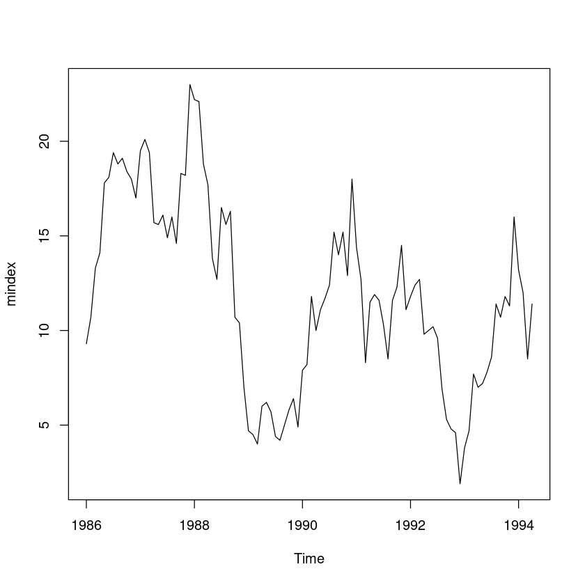

• 추세도 없고 계절성분도 없으니 단순지수평활을 한다.

모형 단순지수평활법 사용 \(Z_t = \beta_{0,t} + \epsilon_t\)

예측 \(\hat Z_n(l) = w Z_n + (1-w) \hat Z_{n-1}(l)\)

-

초기 예측값 \(Z_1^{(1)}\)은 초기 평활값 \(S_0^{(1)}\)를 사용하여 계산

\(Z_1^{(1)} = S_0^{(1)}=15\)

- w= 0.2

fit0 <- HoltWinters(mindex,
                    alpha = 0.2,
                    beta = FALSE,
                    gamma = FALSE,
                    l.start = 15)

fit0

Holt-Winters exponential smoothing without trend and without seasonal component.

Call:
HoltWinters(x = mindex, alpha = 0.2, beta = FALSE, gamma = FALSE,     l.start = 15.1875)

Smoothing parameters:
 alpha: 0.2
 beta : FALSE
 gamma: FALSE

Coefficients:
      [,1]
a 10.97935

head(cbind(fit0$fitted, mindex))

A Time Series: 6 × 3

	fit0$fitted.xhat	fit0$fitted.level	mindex
Jan 1986	NA	NA	9.3
Feb 1986	15.00000	15.00000	10.7
Mar 1986	14.14000	14.14000	13.3
Apr 1986	13.97200	13.97200	14.1
May 1986	13.99760	13.99760	17.8
Jun 1986	14.75808	14.75808	18.1

• t=2

\(S_2^{(1)} = wZ_2 + (1-w)S_0^{(1)}\)

0.2 * 10.7 + 0.8 * 15

14.14

\(S_3^{(1)} = w Z_3 + w (1-w) Z_2 + (1-w)^2 S_0^{(1)}\)

0.2 * 13.3 + 0.2 * 0.8 * 10.7 + 0.8 * 0.8 * 15

13.972

tail(cbind(fit0$fitted, mindex))

A Time Series: 6 × 3

	fit0$fitted.xhat	fit0$fitted.level	mindex
Nov 1993	9.156768	9.156768	11.3
Dec 1993	9.585414	9.585414	16.0
Jan 1994	10.868331	10.868331	13.2
Feb 1994	11.334665	11.334665	12.0
Mar 1994	11.467732	11.467732	8.5
Apr 1994	10.874186	10.874186	11.4

\(S_{99}^{(1)} = w Z_{99} + w (1-w) Z_{98} + \dots + (1-w)^{100} S_0^{(1)}\)

- 예측 갱신

\[S_n^{(1)} = wZ_n + (1-w)S_{n-1}^{(1)}\]

\(S_{100}^{(1)} = w Z_{100} + (1-w) S_{(99)}^{(1)}\)

0.2 * 11.4 + 0.8 * 10.874186

10.9793488

\(S_{99}^{(1)} = w Z_{99} + (1-w) S_{(98)}^{(1)}\)

0.2 * 8.5 + 0.8 * 11.467732

10.8741856

---

- w = 0.6

fit1 <- HoltWinters(mindex,
                    alpha = 0.6,
                    beta = FALSE,
                    gamma = FALSE,
                    l.start = 15)

fit1

Holt-Winters exponential smoothing without trend and without seasonal component.

Call:
HoltWinters(x = mindex, alpha = 0.6, beta = FALSE, gamma = FALSE,     l.start = 15)

Smoothing parameters:
 alpha: 0.6
 beta : FALSE
 gamma: FALSE

Coefficients:
      [,1]
a 10.90021

head(cbind(fit1$fitted, mindex))

A Time Series: 6 × 3

	fit1$fitted.xhat	fit1$fitted.level	mindex
Jan 1986	NA	NA	9.3
Feb 1986	15.00000	15.00000	10.7
Mar 1986	12.42000	12.42000	13.3
Apr 1986	12.94800	12.94800	14.1
May 1986	13.63920	13.63920	17.8
Jun 1986	16.13568	16.13568	18.1

• t=2

\(S_2^{(1)} = wZ_2 + (1-w)S_0^{(1)}\)

0.6 * 10.7 + 0.4 * 15

12.42

\(S_3^{(1)} = w Z_3 + w (1-w) Z_2 + (1-w)^2 S_0^{(1)}\)

0.6 * 13.3 + 0.6*0.4*10.7 + 0.4*0.4*15

12.948

tail(cbind(fit1$fitted, mindex))

A Time Series: 6 × 3

	fit1$fitted.xhat	fit1$fitted.level	mindex
Nov 1993	11.26423	11.26423	11.3
Dec 1993	11.28569	11.28569	16.0
Jan 1994	14.11428	14.11428	13.2
Feb 1994	13.56571	13.56571	12.0
Mar 1994	12.62628	12.62628	8.5
Apr 1994	10.15051	10.15051	11.4

\(S_{99}^{(1)} = w Z_{99} + w (1-w) Z_{98} + \dots + (1-w)^{100} S_0^{(1)}\)

- 예측 갱신

\[S_n^{(1)} = wZ_n + (1-w)S_{n-1}^{(1)}\]

\(S_{100}^{(1)} = w Z_{100} + (1-w) S_{(99)}^{(1)}\)

0.6*11.4+0.4*10.15051

10.900204

\(S_{99}^{(1)} = w Z_{99} + (1-w) S_{(98)}^{(1)}\)

0.6*8.5+0.4*12.62628

10.150512

---

2 (예측오차분석을 안했다.;;)

(R 실습) 다음의 각 자료에 대해 적절한 평활법을 적용한 후 , 예측오차 분석을 하여 적용한 평활법이 적절했는지 논하여라. 그리고 (2)번의 경우 첫번째 과제 5,6번에서 적합한 모형과 1-시차 후 예측 오차의 제곱합 (SSE) 기준하에서 예측력을 비교하여라.

(1)

‘female.txt’ : 월별 전문기술행정직에 종사하는 여성근로자 수 (단위:명)

female <- scan("female.txt")

fema <- ts(female, start=c(1981,1), frequency=12)

plot(fema)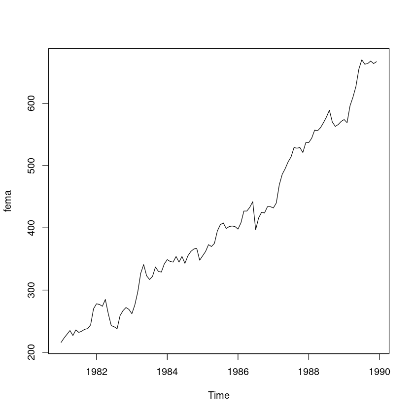

• 시도표를 확인해보니 추세성분과 불규칙성분으로 이루어져 있다. —> 이중지수평활을 사용한다.

- 1모수 이중지수 평활

w <- c(seq(0.1, 0.8, 0.1), seq(0.81, 0.99, 0.01))

df <- data.frame(alpha = numeric(length(w)), beta = numeric(length(w)), sse = numeric(length(w)))
for (i in 1:length(w)) {
  alpha <- w[i]
  beta <- w[i]
  fit <- HoltWinters(fema, alpha = alpha, beta = beta, gamma = FALSE)
  sse <- fit$SSE
  df[i, ] <- c(alpha, beta, sse)
}

df

A data.frame: 27 × 3

alpha	beta	sse
<dbl>	<dbl>	<dbl>
0.10	0.10	47737.16
0.20	0.20	39413.25
0.30	0.30	32655.02
0.40	0.40	28136.56
0.50	0.50	23964.31
0.60	0.60	21390.42
0.70	0.70	20179.01
0.80	0.80	19991.82
0.81	0.81	20034.76
0.82	0.82	20090.85
0.83	0.83	20160.82
0.84	0.84	20245.43
0.85	0.85	20345.55
0.86	0.86	20462.10
0.87	0.87	20596.12
0.88	0.88	20748.74
0.89	0.89	20921.19
0.90	0.90	21114.85
0.91	0.91	21331.22
0.92	0.92	21571.99
0.93	0.93	21839.02
0.94	0.94	22134.40
0.95	0.95	22460.49
0.96	0.96	22819.94
0.97	0.97	23215.75
0.98	0.98	23651.34
0.99	0.99	24130.60

1모수 이중지수일때는 \(\alpha=\beta=0.8\)일 때, SSE값이 19991.82 값을 가진다.

- 이중지수평활 추정

fit_fema <- HoltWinters(fema, gamma=FALSE)

fit_fema

Holt-Winters exponential smoothing with trend and without seasonal component.

Call:
HoltWinters(x = fema, gamma = FALSE)

Smoothing parameters:
 alpha: 1
 beta : 0.01666631
 gamma: FALSE

Coefficients:
        [,1]
a 667.000000
b   5.145043

predict(fit_fema, n.ahead=12, prediction.interval = T, level=0.95) 

A Time Series: 12 × 3

	fit	upr	lwr
Jan 1990	672.1450	694.8066	649.4835
Feb 1990	677.2901	709.6065	644.9736
Mar 1990	682.4351	722.3438	642.5264
Apr 1990	687.5802	734.0440	641.1163
May 1990	692.7252	745.1007	640.3498
Jun 1990	697.8703	755.7139	640.0266
Jul 1990	703.0153	766.0016	640.0290
Aug 1990	708.1603	776.0399	640.2807
Sep 1990	713.3054	785.8813	640.7295
Oct 1990	718.4504	795.5635	641.3374
Nov 1990	723.5955	805.1148	642.0761
Dec 1990	728.7405	814.5572	642.9238

fit_fema$SSE

14153.8104898823

---

- 단순지수평활법 적합

fit_fema2 <- HoltWinters(fema, beta=FALSE, gamma=FALSE)
fit_fema2
fit_fema2$SSE

Holt-Winters exponential smoothing without trend and without seasonal component.

Call:
HoltWinters(x = fema, beta = FALSE, gamma = FALSE)

Smoothing parameters:
 alpha: 0.9999225
 beta : FALSE
 gamma: FALSE

Coefficients:
      [,1]
a 666.9998

15579.4993710227

---

- 계절지수평활법 적합

fit_fema3 <- HoltWinters(fema, seasonal="additive")
fit_fema3
fit_fema3$SSE

Holt-Winters exponential smoothing with trend and additive seasonal component.

Call:
HoltWinters(x = fema, seasonal = "additive")

Smoothing parameters:
 alpha: 0.5689925
 beta : 0.01533418
 gamma: 1

Coefficients:
          [,1]
a   677.319852
b     4.462732
s1  -10.805353
s2  -10.907550
s3   13.687188
s4   21.650246
s5   29.187883
s6   39.477663
s7   33.205948
s8   19.062994
s9    5.235871
s10  -3.290505
s11 -11.437139
s12 -10.319852

25835.5416290603

(2)

‘export.txt’ ; 월별수출액(단위:억$)

export <- scan("export.txt")

expo <- ts(export, start=c(1981,1), frequency=12)

plot.ts(expo)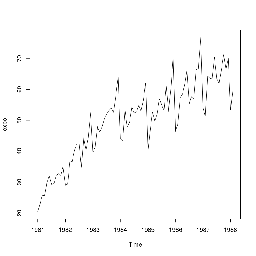

• 추세성분, 계절성분(주기12), 불규칙성분으로 구성되어 있다. –> 계절지수 평활을 이용하자!

- 가법모형

fit_expo_a <- HoltWinters(expo, seasonal="additive") #default는 additive
fit_expo_a

Holt-Winters exponential smoothing with trend and additive seasonal component.

Call:
HoltWinters(x = expo, seasonal = "additive")

Smoothing parameters:
 alpha: 0.3304767
 beta : 0.04369053
 gamma: 0.6102758

Coefficients:
           [,1]
a    66.9300146
b     0.3670945
s1   -0.9590061
s2   -2.3460160
s3   -1.4388022
s4    4.0020957
s5   -2.8546787
s6   -3.1036803
s7    0.4486017
s8    3.3118493
s9    1.6302355
s10   8.0731659
s11 -11.5480012
s12  -8.8892298

fit_expo_m <- HoltWinters(expo, seasonal="multiplicative")
fit_expo_m

Holt-Winters exponential smoothing with trend and multiplicative seasonal component.

Call:
HoltWinters(x = expo, seasonal = "multiplicative")

Smoothing parameters:
 alpha: 0.4285887
 beta : 0.02606259
 gamma: 0.4083356

Coefficients:
          [,1]
a   68.7136998
b    0.5141142
s1   0.9879869
s2   0.9620299
s3   0.9996946
s4   1.0834386
s5   0.9897148
s6   0.9744549
s7   1.0319339
s8   1.0425559
s9   1.0357445
s10  1.1286956
s11  0.8073858
s12  0.8400441

fit_expo_a$SSE

1135.42182593918

fit_expo_m$SSE

1048.2628205778

승법 모형의 SSE가 더 작으니 이 모형을 선택하자.

- 이중지수

fit_expo2<- HoltWinters(expo, gamma=FALSE )
fit_expo2$SSE

3338.93312288425

fit_expo3<- HoltWinters(expo, beta=FALSE, gamma=FALSE )
fit_expo3$SSE

3311.57259808501

hw1_6

z <- scan("export.txt")
n <- length(z)
n

86

z_ts <- ts(z, frequency=12)
cycle(z_ts)

A Time Series: 8 × 12

	Jan	Feb	Mar	Apr	May	Jun	Jul	Aug	Sep	Oct	Nov	Dec
1	1	2	3	4	5	6	7	8	9	10	11	12
2	1	2	3	4	5	6	7	8	9	10	11	12
3	1	2	3	4	5	6	7	8	9	10	11	12
4	1	2	3	4	5	6	7	8	9	10	11	12
5	1	2	3	4	5	6	7	8	9	10	11	12
6	1	2	3	4	5	6	7	8	9	10	11	12
7	1	2	3	4	5	6	7	8	9	10	11	12
8	1	2

seasonal_I <- as.factor(cycle(z_ts))
t <- 1:n
m2 <- lm(z~t+seasonal_I)

summary(m2)

Call:
lm(formula = z ~ t + seasonal_I)

Residuals:
     Min       1Q   Median       3Q      Max 
-10.8562  -2.2938   0.1567   2.6730   9.3951 

Coefficients:
             Estimate Std. Error t value Pr(>|t|)    
(Intercept)  21.98000    1.73500  12.669  < 2e-16 ***
t             0.43721    0.01893  23.097  < 2e-16 ***
seasonal_I2   1.71779    2.16697   0.793 0.430512    
seasonal_I3   9.21741    2.24422   4.107 0.000103 ***
seasonal_I4   7.37163    2.24366   3.286 0.001566 ** 
seasonal_I5   9.30299    2.24326   4.147 8.98e-05 ***
seasonal_I6  12.96578    2.24302   5.780 1.72e-07 ***
seasonal_I7   9.16286    2.24294   4.085 0.000112 ***
seasonal_I8   7.73422    2.24302   3.448 0.000941 ***
seasonal_I9  11.07272    2.24326   4.936 4.88e-06 ***
seasonal_I10 10.68409    2.24366   4.762 9.47e-06 ***
seasonal_I11 12.37545    2.24422   5.514 5.03e-07 ***
seasonal_I12 18.57967    2.24494   8.276 4.26e-12 ***
---
Signif. codes:  0 ‘***’ 0.001 ‘**’ 0.01 ‘*’ 0.05 ‘.’ 0.1 ‘ ’ 1

Residual standard error: 4.334 on 73 degrees of freedom
Multiple R-squared:  0.9011,    Adjusted R-squared:  0.8848 
F-statistic:  55.4 on 12 and 73 DF,  p-value: < 2.2e-16

SSE <- sum(m2$residuals^2)
SSE

1371.05731181319

과제 1에서 적합한 선형모델보다 평활법(계절지수, 가법_승법_)으로 적합한 모델의 SSE가 너 낮게 나왔다.

3

(R 실습) ’data1.csv’는 모의 실험에 의해 생성된 시계열자료(t:시간, z:시계열자료)이다.다음 물음 에 답하여라.

data1 <- read.csv("data1.csv")
t <- data1$t
y <- data1$z
z <- cbind(x,y)
n <- length(data1$t)
data1_ <- ts(y, start=c(1981,1),frequency=12)
data1_

A Time Series: 9 × 12

	Jan	Feb	Mar	Apr	May	Jun	Jul	Aug	Sep	Oct	Nov	Dec
1981	-1.5346871	2.6850469	-0.4288189	1.3724199	-0.9800884	2.4156505	0.1460579	1.9565546	0.3314012	0.1031952	4.5465702	3.3733991
1982	2.1320092	1.4610979	3.5995999	2.6229617	3.3260846	2.6279068	2.4061911	4.9681833	2.1537724	3.2376604	2.0848844	4.4146009
1983	5.5427871	3.5727733	3.6793795	1.0197987	4.1619256	3.9038326	2.1724542	4.9360919	4.8127781	4.6404884	4.4090738	3.3529045
1984	4.0967541	3.4881527	4.4249974	4.3210561	7.7103219	5.0907609	4.5999605	4.9773808	7.6107690	4.9986647	7.1678722	7.1542270
1985	6.6329637	2.8462231	9.3646617	4.4855729	5.2444451	5.8160173	5.0466196	9.5742821	9.0751720	6.6775546	6.7345322	5.7569890
1986	8.3008035	7.5701959	6.5050066	6.0962461	7.4245090	4.4973441	6.5920516	6.9026479	4.6123368	7.7952478	8.4416974	5.6684225
1987	8.5028659	8.8312543	6.9776594	7.0775957	8.4638087	10.7761422	9.4661818	8.7774843	8.9804188	7.1654550	9.5367387	8.8641697
1988	8.9645710	7.5418683	9.0336999	10.8611356	8.7190544	14.1133979	9.5868440	11.4598053	8.2142746	10.9960972	11.3776375	11.4480245
1989	12.5356509	8.8132146	9.1437447	10.2114895

plot(data1_)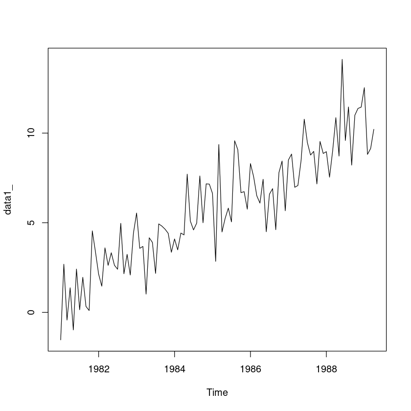

• 추세와 계절성분, 불규칙성이 있어보인다.

(1) 교수님은 계절성분이 없고 추세만 있어 모형을 적합하였음

적절한 추세 모형을 적합시킨 후 잔차분석을 하여라.

계절추세모형 \[Z_t = \beta_0 + \beta_1 + \sum_{i=1}^l 2\delta_i \times I_{tl} + \epsilon_t$, 단 $\delta_1=0\]

cycle(data1_)

A Time Series: 9 × 12

	Jan	Feb	Mar	Apr	May	Jun	Jul	Aug	Sep	Oct	Nov	Dec
1981	1	2	3	4	5	6	7	8	9	10	11	12
1982	1	2	3	4	5	6	7	8	9	10	11	12
1983	1	2	3	4	5	6	7	8	9	10	11	12
1984	1	2	3	4	5	6	7	8	9	10	11	12
1985	1	2	3	4	5	6	7	8	9	10	11	12
1986	1	2	3	4	5	6	7	8	9	10	11	12
1987	1	2	3	4	5	6	7	8	9	10	11	12
1988	1	2	3	4	5	6	7	8	9	10	11	12
1989	1	2	3	4

seasonal_I <- as.factor(cycle(data1_))
#t <- 1:n
m2 <- lm(y~ 0+ t +seasonal_I)

summary(m2)

Call:
lm(formula = y ~ 0 + t + seasonal_I)

Residuals:
    Min      1Q  Median      3Q     Max 
-3.4526 -0.8739 -0.1227  0.8747  3.7703 

Coefficients:
             Estimate Std. Error t value Pr(>|t|)    
t             0.09971    0.00507  19.667  < 2e-16 ***
seasonal_I1   1.24446    0.54646   2.277  0.02522 *  
seasonal_I2   0.21542    0.54878   0.393  0.69562    
seasonal_I3   0.72572    0.55115   1.317  0.19138    
seasonal_I4   0.15582    0.55354   0.282  0.77899    
seasonal_I5   0.82223    0.56859   1.446  0.15175    
seasonal_I6   1.36889    0.57074   2.398  0.01860 *  
seasonal_I7   0.11609    0.57292   0.203  0.83990    
seasonal_I8   1.70838    0.57513   2.970  0.00384 ** 
seasonal_I9   0.63848    0.57739   1.106  0.27185    
seasonal_I10  0.51670    0.57967   0.891  0.37519    
seasonal_I11  1.50257    0.58200   2.582  0.01150 *  
seasonal_I12  0.86957    0.58436   1.488  0.14035    
---
Signif. codes:  0 ‘***’ 0.001 ‘**’ 0.01 ‘*’ 0.05 ‘.’ 0.1 ‘ ’ 1

Residual standard error: 1.46 on 87 degrees of freedom
Multiple R-squared:  0.9584,    Adjusted R-squared:  0.9522 
F-statistic: 154.2 on 13 and 87 DF,  p-value: < 2.2e-16

• 적합모형

\(\hat Z_t = 0.09971 t +1.24446 I_{t1} \dots +0.86957 I_{t12}\)

- 잔차검정

resid_m <- resid(m2)
plot(resid_m, pch=16, type='l')
abline(h=0, lty=2)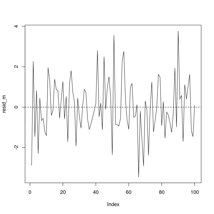

t.test(resid_m)

    One Sample t-test

data:  resid_m
t = 4.1891e-18, df = 99, p-value = 1
alternative hypothesis: true mean is not equal to 0
95 percent confidence interval:
 -0.2716042  0.2716042
sample estimates:
   mean of x 
5.734074e-19 

bptest(m2)

    studentized Breusch-Pagan test

data:  m2
BP = 11.4, df = 12, p-value = 0.495

hist(resid_m)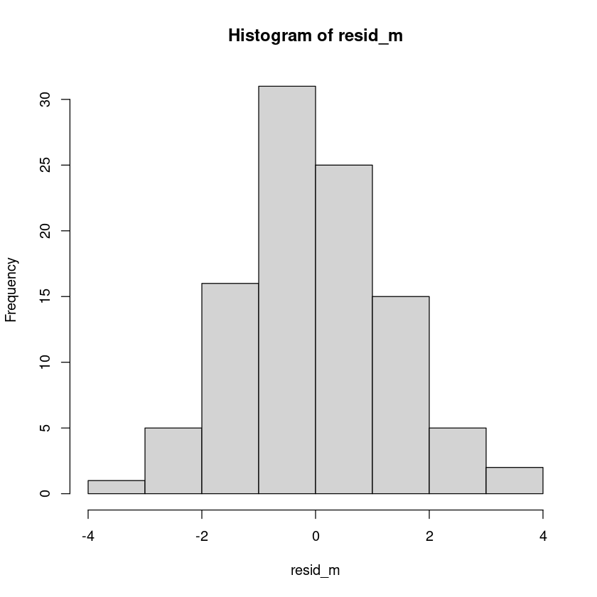

shapiro.test(resid_m)

    Shapiro-Wilk normality test

data:  resid_m
W = 0.99218, p-value = 0.8338

dwtest(m2, alternative = "two.sided") 

    Durbin-Watson test

data:  m2
DW = 2.1153, p-value = 0.5919
alternative hypothesis: true autocorrelation is not 0

(2)

(1)에서 적합한 추세모형에서 1∼ 10 시차 후의 예측값을 구하여라.

new_dt <- data.frame( t = n + (1:10),
 seasonal_I = as.factor(c(5:12,1,2)))
new_dt

A data.frame: 10 × 2

t	seasonal_I
<int>	<fct>
101	5
102	6
103	7
104	8
105	9
106	10
107	11
108	12
109	1
110	2

predict(m2, new_dt)

1

10.8932810379944

2

11.539654967107

3

10.386568516118

4

12.0785772090589

5

11.108388789967

6

11.0863188261925

7

12.1718992420353

8

11.6386155761184

9

12.113216954006

10

11.1838957059557

a <- predict(m2, new_dt)

(3)

적절한 평활법을 적용한 후 잔차분석을 하여라.

• 시도표에서 등분산으로 보이니 가법모형 적용

fit_data_a <- HoltWinters(data1_, seasonal="additive")
fit_data_a

Holt-Winters exponential smoothing with trend and additive seasonal component.

Call:
HoltWinters(x = data1_, seasonal = "additive")

Smoothing parameters:
 alpha: 0.1075626
 beta : 0.03407311
 gamma: 0.2315828

Coefficients:
           [,1]
a   11.19913122
b    0.10780161
s1  -0.07016081
s2   0.66130312
s3  -0.85496062
s4   0.47657925
s5  -0.88090464
s6  -0.76891779
s7   0.57746908
s8  -0.22134249
s9   0.45302226
s10 -1.33334803
s11 -0.44879394
s12 -0.72310382

ls(fit_data_a)

1. 'alpha'
2. 'beta'
3. 'call'
4. 'coefficients'
5. 'fitted'
6. 'gamma'
7. 'seasonal'
8. 'SSE'
9. 'x'

fit_data_a$SSE

241.40429231834

f_resid_m <- resid(fit_data_a)
plot(f_resid_m, pch=16, type='l')
abline(h=0, lty=2)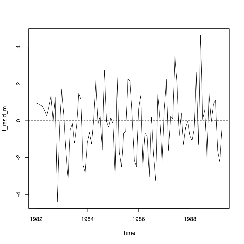

t.test(f_resid_m)

    One Sample t-test

data:  f_resid_m
t = -0.97545, df = 87, p-value = 0.332
alternative hypothesis: true mean is not equal to 0
95 percent confidence interval:
 -0.5232992  0.1787545
sample estimates:
 mean of x 
-0.1722723 

hist(f_resid_m)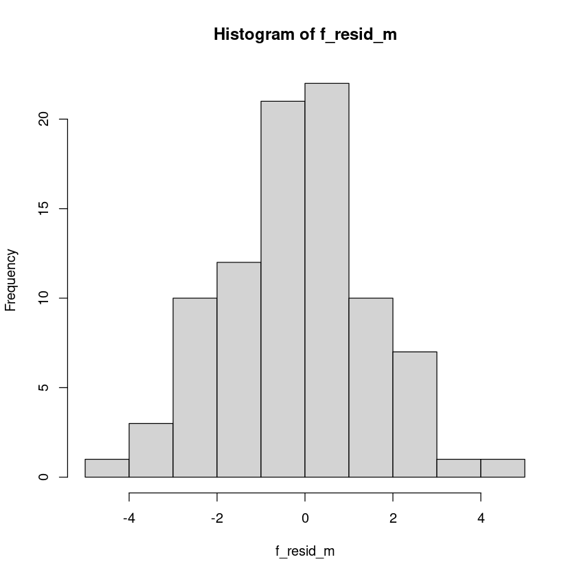

shapiro.test(f_resid_m)

    Shapiro-Wilk normality test

data:  f_resid_m
W = 0.99387, p-value = 0.9586

(4)

(3)의 결과를 이용하여 1∼10시차 후의 예측값을 구하여라.

predict(fit_data_a, n.ahead=10, prediction.interval = T, level=0.95)

A Time Series: 10 × 3

	fit	upr	lwr
May 1989	11.23677	14.48390	7.989648
Jun 1989	12.07604	15.34319	8.808889
Jul 1989	10.66758	13.95596	7.379195
Aug 1989	12.10692	15.41775	8.796079
Sep 1989	10.85723	14.19177	7.522695
Oct 1989	11.07702	14.43652	7.717522
Nov 1989	12.53121	15.91695	9.145475
Dec 1989	11.84020	15.25346	8.426943
Jan 1990	12.62237	16.06444	9.180291
Feb 1990	10.94380	14.41600	7.471600

prediction_result <- predict(fit_data_a, n.ahead=10, prediction.interval = T, level=0.95)

b <- prediction_result[1:10]

(5)

실제 1, 2, . . . , 10 시차 후의 관측값이 ’data1 new.csv’일 때, (2), (4)의 결과를 이용하여 어느 모형이 더 적합했는지에 대해 비교하여라.

data1new <- read.csv("data1_new.csv")

sum((data1new$z - a)^2)

38.302781319433

sum((data1new$z - b)^2)

35.5553155409459

(4)의 모형이 더 적합했다.

CH04

4

(R 실습) ’export.txt’자료에 대하여 각가 다음 물음에 답하여라.

z <- scan("export.txt")
t <- 1:length(z)
export <- ts(z, start=c(1981,1), frequency=12)
plot.ts(export, lwd=2, main="TS plot for export data")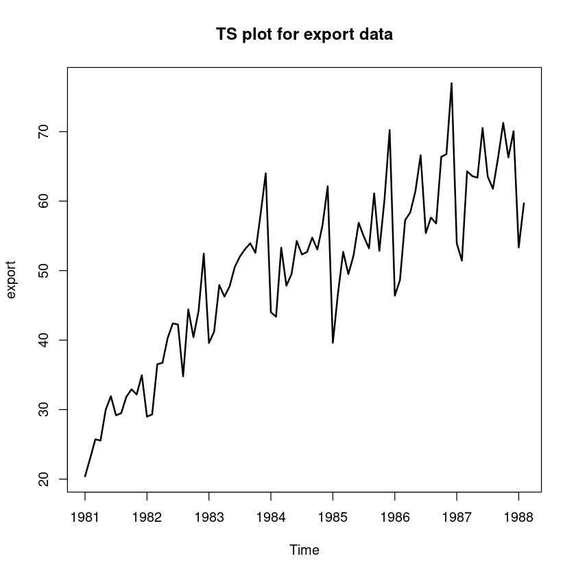

(1)

추세분석을 이용한 분해법에 의한 각 성분의 시계열 그림을 그려라.

- 추세성분 추정: \(Z_t = \beta_0 + \beta_1t + \epsilon_t\) 적합

fit0 <- lm(export  ~ t)
summary(fit0)

Call:
lm(formula = export ~ t)

Residuals:
     Min       1Q   Median       3Q      Max 
-15.1230  -4.0245  -0.6699   4.1819  17.3619 

Coefficients:
            Estimate Std. Error t value Pr(>|t|)    
(Intercept) 30.62075    1.37454   22.28   <2e-16 ***
t            0.44520    0.02744   16.22   <2e-16 ***
---
Signif. codes:  0 ‘***’ 0.001 ‘**’ 0.01 ‘*’ 0.05 ‘.’ 0.1 ‘ ’ 1

Residual standard error: 6.318 on 84 degrees of freedom
Multiple R-squared:  0.758, Adjusted R-squared:  0.7552 
F-statistic: 263.2 on 1 and 84 DF,  p-value: < 2.2e-16

\(\hat T_t = 30.621 + 0.445 t\)

hat_Tt <- fitted(fit0)
ts.plot(export, hat_Tt,
     col=1:2,
     lty=1:2,
     lwd=2:3,
     ylab="export", xlab="time",
     main="시계열과 분해법에 의한 추세성분")
legend("topleft", lty=1:2, col=1:2, lwd=2:3, c("z", "추세성분"))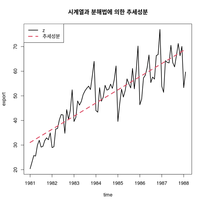

- 계절성분

## 원시계열에서 추세성분 조정
adjtrend_ = export-hat_Tt
plot.ts(adjtrend_, lwd=2)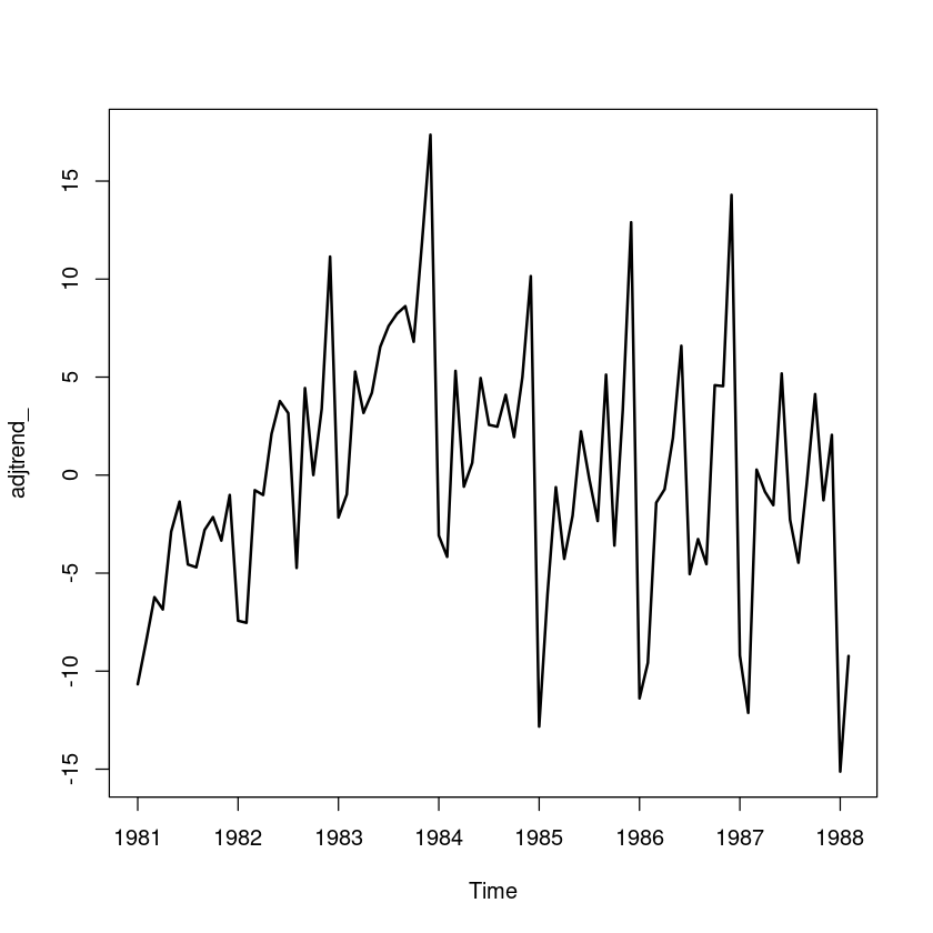

y = factor(cycle(adjtrend_))
fit1 <- lm(adjtrend_ ~ 0+y)  # 제약조건 beta0=0
summary(fit1)

Call:
lm(formula = adjtrend_ ~ 0 + y)

Residuals:
     Min       1Q   Median       3Q      Max 
-10.5684  -2.4909   0.0174   2.5296   9.4910 

Coefficients:
    Estimate Std. Error t value Pr(>|t|)    
y1   -8.9845     1.5237  -5.897 1.03e-07 ***
y2   -7.2747     1.5237  -4.774 8.87e-06 ***
y3    0.2649     1.6289   0.163   0.8713    
y4   -1.5889     1.6289  -0.975   0.3325    
y5    0.3345     1.6289   0.205   0.8379    
y6    3.9893     1.6289   2.449   0.0167 *  
y7    0.1784     1.6289   0.110   0.9131    
y8   -1.2583     1.6289  -0.772   0.4423    
y9    2.0722     1.6289   1.272   0.2073    
y10   1.6756     1.6289   1.029   0.3070    
y11   3.3590     1.6289   2.062   0.0427 *  
y12   9.5552     1.6289   5.866 1.17e-07 ***
---
Signif. codes:  0 ‘***’ 0.001 ‘**’ 0.01 ‘*’ 0.05 ‘.’ 0.1 ‘ ’ 1

Residual standard error: 4.31 on 74 degrees of freedom
Multiple R-squared:  0.5901,    Adjusted R-squared:  0.5236 
F-statistic: 8.878 on 12 and 74 DF,  p-value: 3.121e-10

\(\hat S_t = -8.9845 I_1 + \dots +9.5552I_{12}\)

hat_St <- fitted(fit1)
ts.plot(hat_St, main="추정된 계절성분")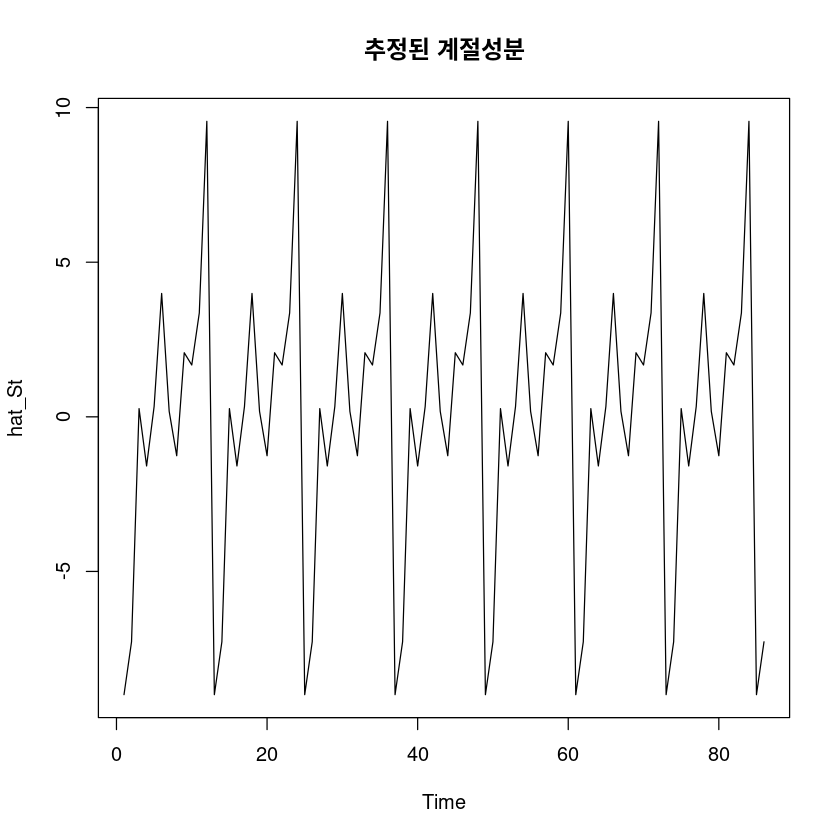

- 불규칙성분

hat_It <- export - hat_Tt - hat_St
ts.plot(hat_It); abline(h=0)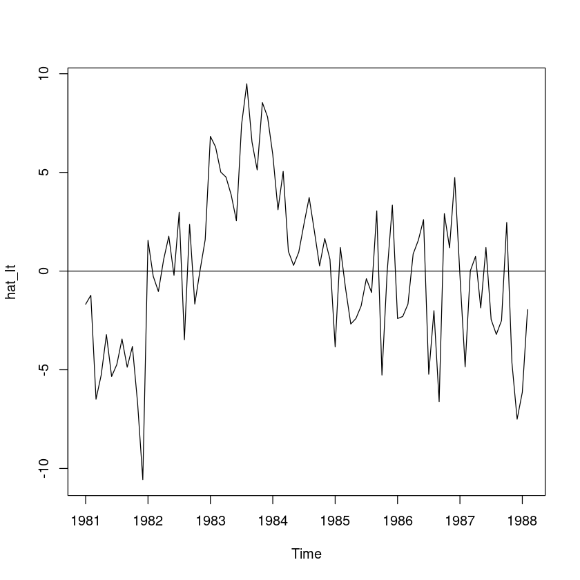

- 추정

pred_a <- hat_Tt + hat_St

ts.plot(export, pred_a, col=1:2, lty=1:2, lwd=2:3,ylab="export", xlab="time")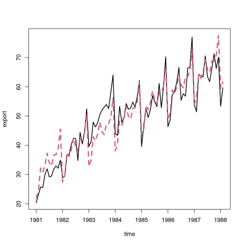

sum((export-pred_a)^2)

1374.40699758301

(2)

추정된 불규칙성분의 분석을 통해 적용된 분해법이 적절했는지 논하여라.

t.test(hat_It) #H0 : mu=E(It)=0

    One Sample t-test

data:  hat_It
t = 8.2505e-16, df = 85, p-value = 1
alternative hypothesis: true mean is not equal to 0
95 percent confidence interval:
 -0.8621323  0.8621323
sample estimates:
   mean of x 
3.577489e-16 

• 평균이 0이다.

hist(hat_It)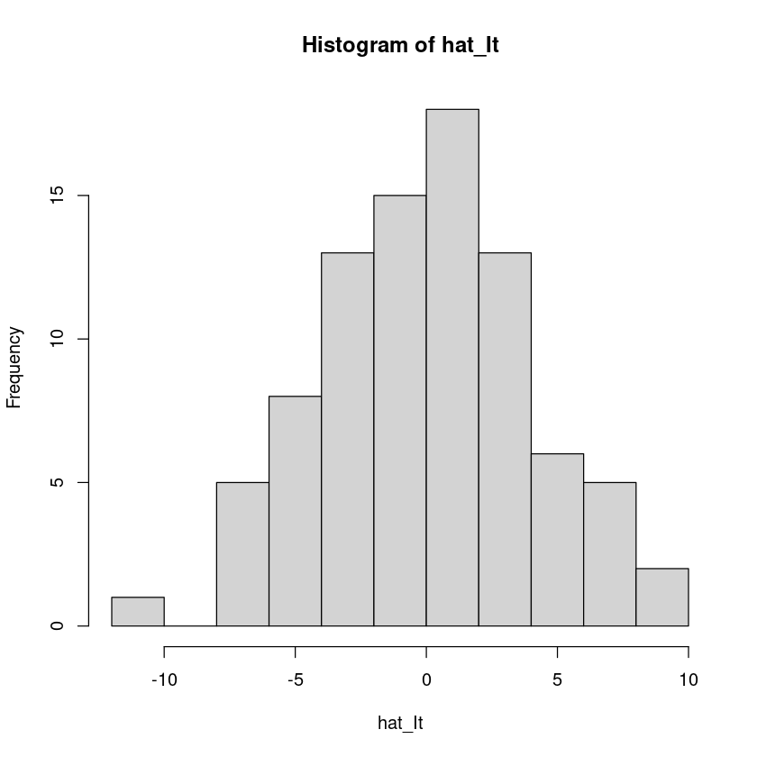

dwtest(lm(hat_It~ t),
 alternative = 'two.sided')

    Durbin-Watson test

data:  lm(hat_It ~ t)
DW = 0.79194, p-value = 1.672e-10
alternative hypothesis: true autocorrelation is not 0

양의 상관관계가 있어보인다.

bptest(lm(hat_It ~ t, data = export))

    studentized Breusch-Pagan test

data:  lm(hat_It ~ t, data = export)
BP = 4.276, df = 1, p-value = 0.03865

(3)

이동평균을 이용한 분해법에 의한 각 성분의 시계열 그림을 그려라

이동평균분해법

z <- scan("export.txt")
t <- 1:length(z)
export <- ts(z, start=c(1981,1), frequency=12)
#plot.ts(export, lwd=2, main="TS plot for export data")
plot.ts(export)
lines(ma(export,3), col='blue', lwd=2)
lines(ma(export,12), col='red', lwd=2)
legend('topleft', lty=c(1,1,1), col=c('black', 'blue', 'red'),
     lwd=c(1,1,2),
     c('원시계열', "CSMA(m=3)", "CSMA(m=12)"),
     bty='n')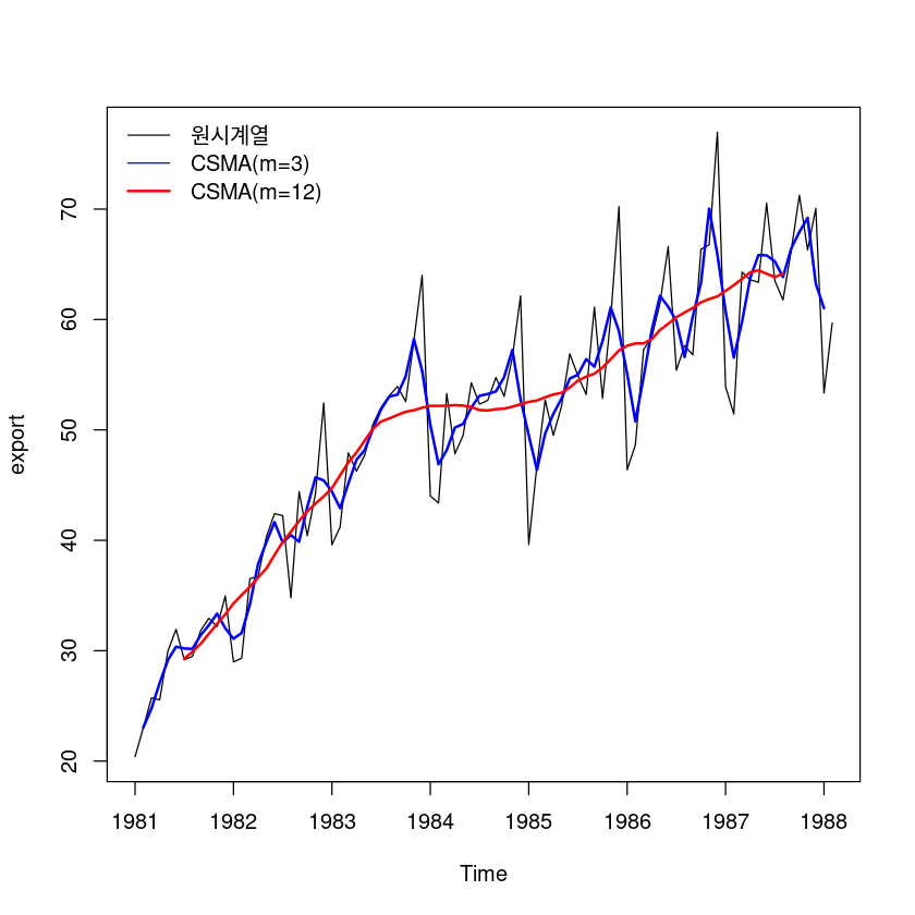

trend = ma(export, 12)
plot.ts(trend, lwd=2)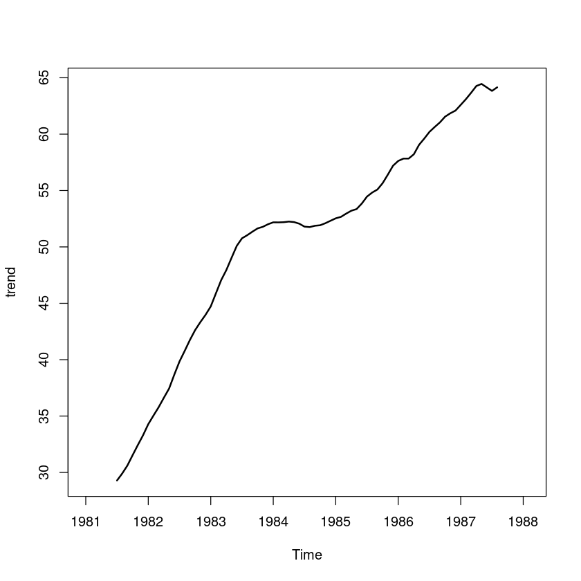

adj_trend <-export - trend
plot.ts(adj_trend, lwd=2)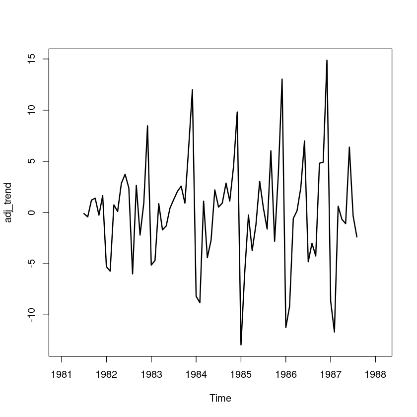

seasonal <- tapply(adj_trend, cycle(adj_trend), function(y) mean(y,na.rm=T))
seasonal

1

-8.57347222222222

2

-7.65451388888889

3

0.41888888888889

4

-1.69965277777778

5

-0.174375000000001

6

3.79819444444445

7

-0.0849999999999983

8

-1.4907738095238

9

1.85138888888889

10

0.540972222222225

11

3.35631944444444

12

9.97465277777778

summary(lm(adj_trend~0+as.factor(cycle(adj_trend))))

Call:
lm(formula = adj_trend ~ 0 + as.factor(cycle(adj_trend)))

Residuals:
    Min      1Q  Median      3Q     Max 
-8.3226 -1.4141  0.3492  1.8005  4.9008 

Coefficients:
                              Estimate Std. Error t value Pr(>|t|)    
as.factor(cycle(adj_trend))1   -8.5735     1.1268  -7.608 1.89e-10 ***
as.factor(cycle(adj_trend))2   -7.6545     1.1268  -6.793 4.90e-09 ***
as.factor(cycle(adj_trend))3    0.4189     1.1268   0.372  0.71135    
as.factor(cycle(adj_trend))4   -1.6997     1.1268  -1.508  0.13654    
as.factor(cycle(adj_trend))5   -0.1744     1.1268  -0.155  0.87752    
as.factor(cycle(adj_trend))6    3.7982     1.1268   3.371  0.00129 ** 
as.factor(cycle(adj_trend))7   -0.0850     1.0432  -0.081  0.93533    
as.factor(cycle(adj_trend))8   -1.4908     1.0432  -1.429  0.15803    
as.factor(cycle(adj_trend))9    1.8514     1.1268   1.643  0.10544    
as.factor(cycle(adj_trend))10   0.5410     1.1268   0.480  0.63286    
as.factor(cycle(adj_trend))11   3.3563     1.1268   2.979  0.00413 ** 
as.factor(cycle(adj_trend))12   9.9747     1.1268   8.852 1.33e-12 ***
---
Signif. codes:  0 ‘***’ 0.001 ‘**’ 0.01 ‘*’ 0.05 ‘.’ 0.1 ‘ ’ 1

Residual standard error: 2.76 on 62 degrees of freedom
  (12 observations deleted due to missingness)
Multiple R-squared:  0.7721,    Adjusted R-squared:  0.728 
F-statistic:  17.5 on 12 and 62 DF,  p-value: 1.335e-15

mean(seasonal)

0.021885747354499

seasonal <- seasonal - mean(seasonal) #평균을 0으로 수정
seasonal

1

-8.59535796957672

2

-7.67639963624339

3

0.397003141534391

4

-1.72153852513228

5

-0.1962607473545

6

3.77630869708995

7

-0.106885747354497

8

-1.5126595568783

9

1.82950314153439

10

0.519086474867726

11

3.33443369708995

12

9.95276703042328

St = rep(seasonal, 7)
plot.ts(St)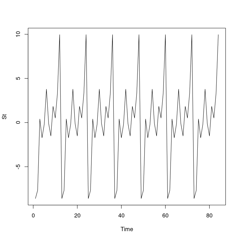

irregular <- export - trend - St
plot.ts(irregular)
abline(h=0, lty=2)

Warning message in `-.default`(export - trend, St):
“longer object length is not a multiple of shorter object length”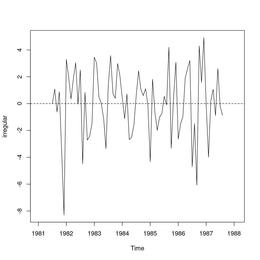

decompose 함수 이용

dec_fit <- decompose(export, 'additive')
dec_fit

$x
       Jan   Feb   Mar   Apr   May   Jun   Jul   Aug   Sep   Oct   Nov   Dec
1981 20.40 23.01 25.73 25.55 29.96 31.94 29.18 29.48 31.83 32.93 32.18 34.95
1982 28.98 29.32 36.53 36.73 40.29 42.41 42.24 34.79 44.41 40.42 44.24 52.45
1983 39.59 41.21 47.92 46.26 47.73 50.52 52.03 53.10 53.93 52.56 58.10 64.01
1984 44.01 43.37 53.30 47.84 49.50 54.27 52.33 52.68 54.75 53.04 56.55 62.14
1985 39.61 46.80 52.71 49.50 52.15 56.89 54.90 53.21 61.12 52.85 60.20 70.23
1986 46.39 48.65 57.26 58.39 61.46 66.60 55.40 57.63 56.80 66.37 66.77 76.97
1987 53.92 51.44 64.29 63.61 63.37 70.53 63.52 61.77 66.25 71.26 66.29 70.07
1988 53.34 59.68                                                            

$seasonal
            Jan        Feb        Mar        Apr        May        Jun
1981 -8.5953580 -7.6763996  0.3970031 -1.7215385 -0.1962607  3.7763087
1982 -8.5953580 -7.6763996  0.3970031 -1.7215385 -0.1962607  3.7763087
1983 -8.5953580 -7.6763996  0.3970031 -1.7215385 -0.1962607  3.7763087
1984 -8.5953580 -7.6763996  0.3970031 -1.7215385 -0.1962607  3.7763087
1985 -8.5953580 -7.6763996  0.3970031 -1.7215385 -0.1962607  3.7763087
1986 -8.5953580 -7.6763996  0.3970031 -1.7215385 -0.1962607  3.7763087
1987 -8.5953580 -7.6763996  0.3970031 -1.7215385 -0.1962607  3.7763087
1988 -8.5953580 -7.6763996                                            
            Jul        Aug        Sep        Oct        Nov        Dec
1981 -0.1068857 -1.5126596  1.8295031  0.5190865  3.3344337  9.9527670
1982 -0.1068857 -1.5126596  1.8295031  0.5190865  3.3344337  9.9527670
1983 -0.1068857 -1.5126596  1.8295031  0.5190865  3.3344337  9.9527670
1984 -0.1068857 -1.5126596  1.8295031  0.5190865  3.3344337  9.9527670
1985 -0.1068857 -1.5126596  1.8295031  0.5190865  3.3344337  9.9527670
1986 -0.1068857 -1.5126596  1.8295031  0.5190865  3.3344337  9.9527670
1987 -0.1068857 -1.5126596  1.8295031  0.5190865  3.3344337  9.9527670
1988                                                                  

$trend
          Jan      Feb      Mar      Apr      May      Jun      Jul      Aug
1981       NA       NA       NA       NA       NA       NA 29.28583 29.90625
1982 34.27833 35.04375 35.78917 36.62542 37.44000 38.67167 39.84292 40.78042
1983 44.72292 45.89375 47.05333 47.95583 49.03917 50.09833 50.76417 51.03833
1984 52.18083 52.17583 52.19250 52.24667 52.20208 52.05958 51.79833 51.75792
1985 52.53625 52.66542 52.95292 53.21042 53.35458 53.84375 54.46333 54.82292
1986 57.62583 57.83083 57.83500 58.21833 59.05542 59.61000 60.20458 60.63458
1987 62.59667 63.10750 63.67375 64.27125 64.45500 64.14750 63.83583 64.15500
1988       NA       NA                                                      
          Sep      Oct      Nov      Dec
1981 30.61917 31.53500 32.43125 33.29792
1982 41.75042 42.62208 43.32917 43.97708
1983 51.35250 51.64250 51.78208 52.01208
1984 51.87625 51.92083 52.10042 52.32000
1985 55.08958 55.64958 56.40792 57.20042
1986 61.04375 61.55417 61.85125 62.09458
1987       NA       NA       NA       NA
1988                                    

$random
              Jan          Feb          Mar          Apr          May
1981           NA           NA           NA           NA           NA
1982  3.297024636  1.952649636  0.343830192  1.826121858  3.046260747
1983  3.462441303  2.992649636  0.469663525  0.025705192 -1.112905919
1984  0.424524636 -1.129433697  0.710496858 -2.685128142 -2.505822586
1985 -4.330892030  1.810982970 -0.639919808 -1.988878142 -1.008322586
1986 -2.640475364 -1.504433697 -0.972003142  1.893205192  2.600844081
1987 -0.081308697 -3.991100364  0.219246858  1.060288525 -0.888739253
1988           NA           NA                                       
              Jun          Jul          Aug          Sep          Oct
1981           NA  0.001052414  1.086409557 -0.618669808  0.875913525
1982 -0.037975364  2.503969081 -4.477757110  0.830080192 -2.721169808
1983 -3.354642030  1.372719081  3.574326224  0.747996858  0.398413525
1984 -1.565892030  0.638552414  2.434742890  1.044246858  0.600080192
1985 -0.730058697  0.543552414 -0.100257110  4.200913525 -3.318669808
1986  3.213691303 -4.697697586 -1.491923776 -6.073253142  4.296746858
1987  2.606191303 -0.208947586 -0.872340443           NA           NA
1988                                                                 
              Nov          Dec
1981 -3.585683697 -8.300683697
1982 -2.423600364 -1.479850364
1983  2.983482970  2.045149636
1984  1.115149636 -0.132767030
1985  0.457649636  3.076816303
1986  1.584316303  4.922649636
1987           NA           NA
1988                          

$figure
 [1] -8.5953580 -7.6763996  0.3970031 -1.7215385 -0.1962607  3.7763087
 [7] -0.1068857 -1.5126596  1.8295031  0.5190865  3.3344337  9.9527670

$type
[1] "additive"

attr(,"class")
[1] "decomposed.ts"

plot(dec_fit)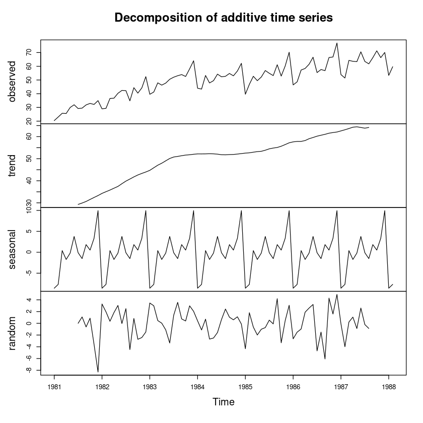

dec_fit2 <- decompose(export, type = "multiplicative")
plot(dec_fit2)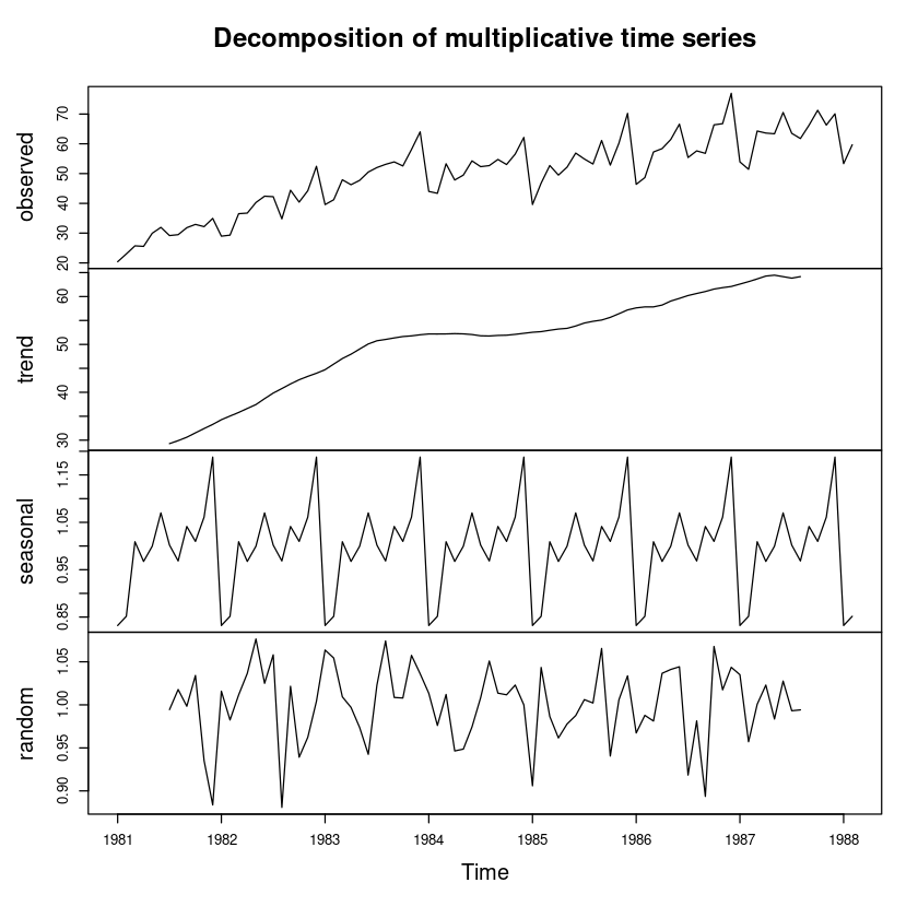

## 가법모형 vs. 승법모형
pred_dec <-dec_fit$trend+dec_fit$seasonal
pred_dec2 <-dec_fit2$trend*dec_fit2$seasonal

ts.plot(pred_dec, pred_dec2, col=1:2, lty=1:2, ylab="food", xlab="time")
legend("topleft", lty=1:2, col=1:2, c("가법모형", "승법모형"))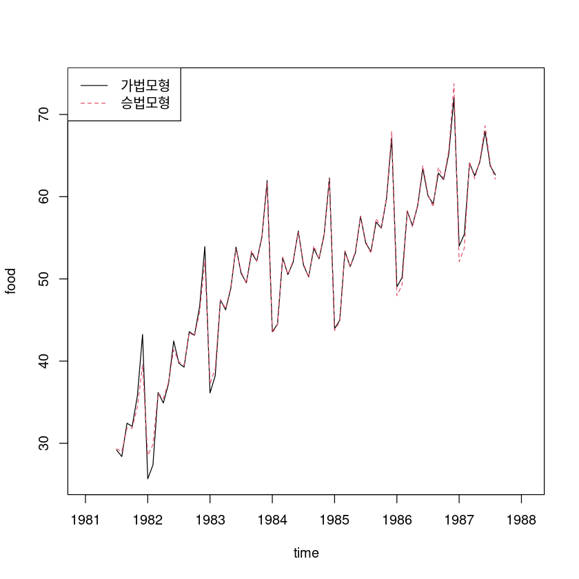

stl함수 이용

stl_fit1 <- stl(export, s.window=12)
stl_fit1

 Call:
 stl(x = export, s.window = 12)

Components
            seasonal    trend    remainder
Jan 1981 -8.03824134 26.81776  1.620485206
Feb 1981 -6.63002814 27.30969  2.330333480
Mar 1981 -0.13110622 27.80163 -1.940526967
Apr 1981 -2.16782904 28.29357 -0.575742678
May 1981 -0.02387280 28.83742  1.146455416
Jun 1981  3.12006392 29.38126 -0.561326978
Jul 1981  0.19259616 29.92511 -0.937704893
Aug 1981 -1.39615399 30.52457  0.351588714
Sep 1981  2.08889246 31.12402 -1.382914272
Oct 1981  0.78594126 31.72348  0.420580381
Nov 1981  3.14306515 32.53144 -3.494505630
Dec 1981  9.25329283 33.33940 -7.642695428
Jan 1982 -8.18853645 34.14736  3.021171726
Feb 1982 -6.74205914 35.02084  1.041217119
Mar 1982 -0.11359668 35.89432  0.749277352
Apr 1982 -2.14642909 36.76780  2.108632461
May 1982 -0.04765717 37.74653  2.591125433
Jun 1982  3.22089766 38.72527  0.463835494
Jul 1982  0.10549237 39.70400  2.430505678
Aug 1982 -1.41993463 40.61875 -4.408810621
Sep 1982  2.04045104 41.53349  0.836060406
Oct 1982  0.89651488 42.44823 -2.924746731
Nov 1982  3.20038177 43.30548 -2.265858677
Dec 1982  9.40282354 44.16272 -1.115545502
Jan 1983 -8.33955445 45.01997  2.909587433
Feb 1983 -6.85397510 46.00456  2.059414793
Mar 1983 -0.09513416 46.98915  1.025980554
Apr 1983 -2.12310901 47.97375  0.409362112
May 1983 -0.06855425 48.79308 -0.994521923
Jun 1983  3.32542520 49.61241 -2.417830650
Jul 1983  0.02288888 50.43173  1.575376391
Aug 1983 -1.43898388 50.82162  3.717366595
Sep 1983  1.99697212 51.21150  0.721528047
Oct 1983  1.01133498 51.60138 -0.052717360
Nov 1983  3.26122886 51.76546  3.073314934
Dec 1983  9.55393181 51.92953  2.526538154
Jan 1984 -8.63020919 52.09360  0.546605321
Feb 1984 -7.05228753 52.10779 -1.685505543
Mar 1984 -0.02362451 52.12198  1.201642230
Apr 1984 -2.05361665 52.13617 -2.242554829
May 1984 -0.12808589 52.06895 -2.440860110
Jun 1984  3.51447214 52.00172 -1.246192660
Jul 1984 -0.10905922 51.93450  0.504564171
Aug 1984 -1.46691120 51.96370  2.183207296
Sep 1984  1.91927553 51.99291  0.837811709
Oct 1984  1.27127927 52.02212 -0.253400890
Nov 1984  3.36913024 52.18801  0.992858614
Dec 1984  9.78170407 52.35390  0.004395256
Jan 1985 -8.94600253 52.51979 -3.963787671
Feb 1985 -7.27425538 52.75254  1.321719247
Mar 1985  0.02571289 52.98528 -0.300994963
Apr 1985 -2.00432115 53.21803 -1.713706857
May 1985 -0.20583899 53.58938 -1.233544814
Jun 1985  3.68735310 53.96074 -0.758092699
Jul 1985 -0.25511780 54.33210  0.823022411
Aug 1985 -1.50687743 54.83525 -0.118367709
Sep 1985  1.83161162 55.33839  3.949993500
Oct 1985  1.52356468 55.84154 -4.515109315
Nov 1985  3.47168119 56.34545  0.382869321
Dec 1985 10.00699125 56.84935  3.373654404
Jan 1986 -9.17170413 57.35326 -1.791555078
Feb 1986 -7.34995073 57.74972 -1.749772497
Mar 1986  0.01792431 58.14619 -0.904111549
Apr 1986 -2.00925233 58.54265  1.856601080
May 1986 -0.25578936 59.05157  2.664216221
Jun 1986  3.77379354 59.56050  3.265711445
Jul 1986 -0.35038247 60.06942 -4.319034430
Aug 1986 -1.52477949 60.53012 -1.375341107
Sep 1986  1.78721730 60.99082 -5.978041605
Oct 1986  1.64995719 61.45153  3.268514805
Nov 1986  3.51677071 61.86477  1.388457561
Dec 1986 10.11358765 62.27802  4.578396895
Jan 1987 -9.37155076 62.69126  0.600291580
Feb 1987 -7.40218241 63.09442 -4.252233068
Mar 1987  0.03120809 63.49757  0.761220146
Apr 1987 -1.99625213 63.90073  1.705524066
May 1987 -0.29094930 63.96479 -0.303838557
Jun 1987  3.87191769 64.02885  2.629234647
Jul 1987 -0.43707012 64.09291 -0.135837345
Aug 1987 -1.53661763 64.17446 -0.867840726
Sep 1987  1.74637383 64.25601  0.247616920
Oct 1987  1.77824626 64.33756  5.144193599
Nov 1987  3.56210251 64.39946 -1.671565286
Dec 1987 10.21967043 64.46137 -4.611035849
Jan 1988 -9.50110743 64.52327 -1.682160623
Feb 1988 -7.47541608 64.56485  2.590568880

plot(stl_fit1)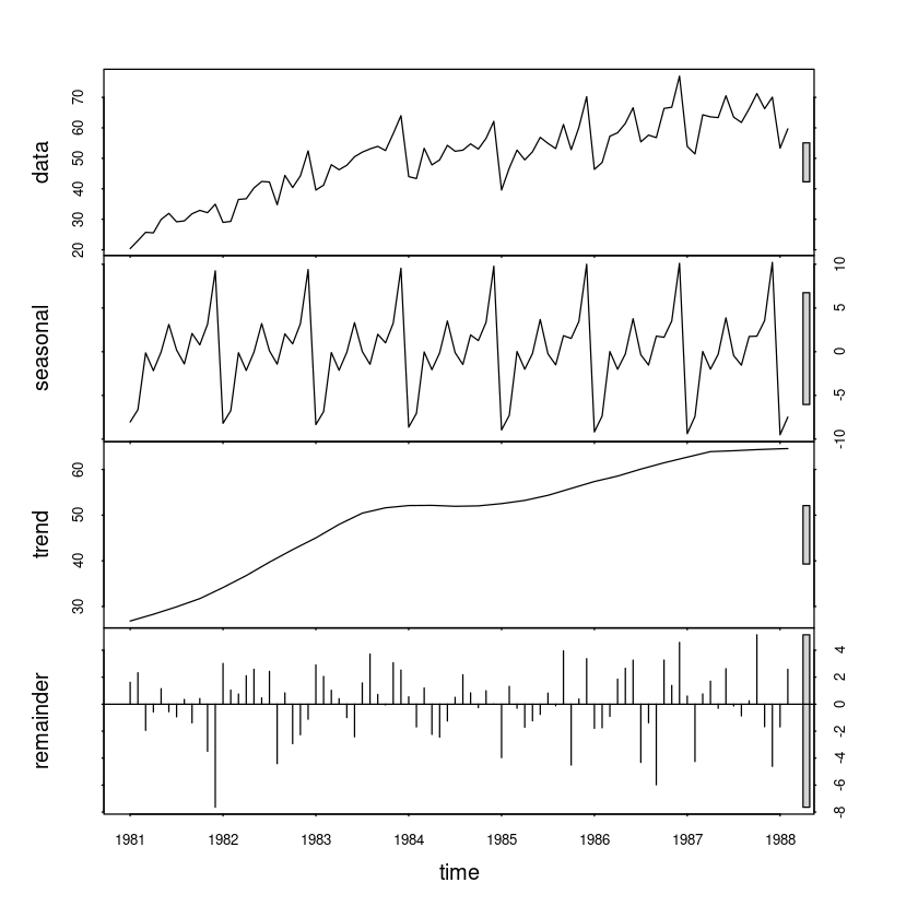

pred_stl <- stl_fit1$time.series[,1]+stl_fit1$time.series[,2]

(4)

추정된 불규칙성분의 분석을 통해 적용된 분해법이 적절했는지 논하여라.

t.test(irregular)

    One Sample t-test

data:  irregular
t = 0.074013, df = 73, p-value = 0.9412
alternative hypothesis: true mean is not equal to 0
95 percent confidence interval:
 -0.5674456  0.6112171
sample estimates:
 mean of x 
0.02188575 

dwtest(lm(irregular~1))

    Durbin-Watson test

data:  lm(irregular ~ 1)
DW = 1.9469, p-value = 0.4094
alternative hypothesis: true autocorrelation is greater than 0

dwtest(lm(irregular~t))

    Durbin-Watson test

data:  lm(irregular ~ t)
DW = 1.9477, p-value = 0.3643
alternative hypothesis: true autocorrelation is greater than 0

추정

fit_ <- trend + St
ts.plot(export, fit_, lty=1:2, col=1:2, lwd=2:3)

Warning message in `+.default`(trend, St):
“longer object length is not a multiple of shorter object length”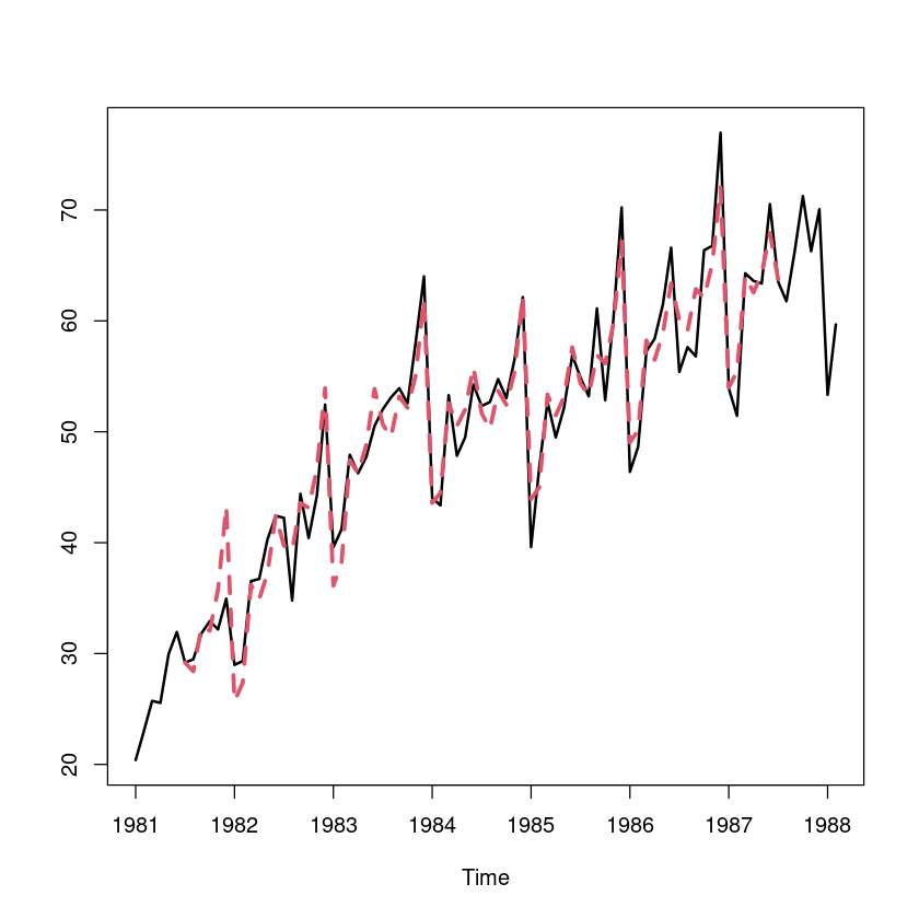

(5)

각 분해법에 의한 결과를 1-시착 후 예측오차의 제곱합 (SSE) 기준하에서 2번의 결과와 예측 력을 비교하여라.

- decompose

sum((export-pred_dec)^2, na.rm=T) #SSE - 가법
sum((export-pred_dec2)^2, na.rm=T) #SSE - 승법

472.381499188028

353.176184412717

- stl

sum((export-pred_stl)^2) 

506.70574427387

5

(R 실습) ’usapass.txt’는 미국 월별 비행기 승객 수(단위 : 천 명)의 시계열자료이다. log 변환 후 아래의 분석을 수행하시오. ((2),(3),(4)번에 대하여 모형을 적합한 후 실제데이터와 각 모형에서 구해진 추정값을 비교하는 그림도 포함)

z5 <- scan("usapass.txt")
t <- 1:length(z5)
usapass <- ts(z5, start=c(1981,1), frequency=12)

plot.ts(usapass, lwd=2, main="TS plot for export data")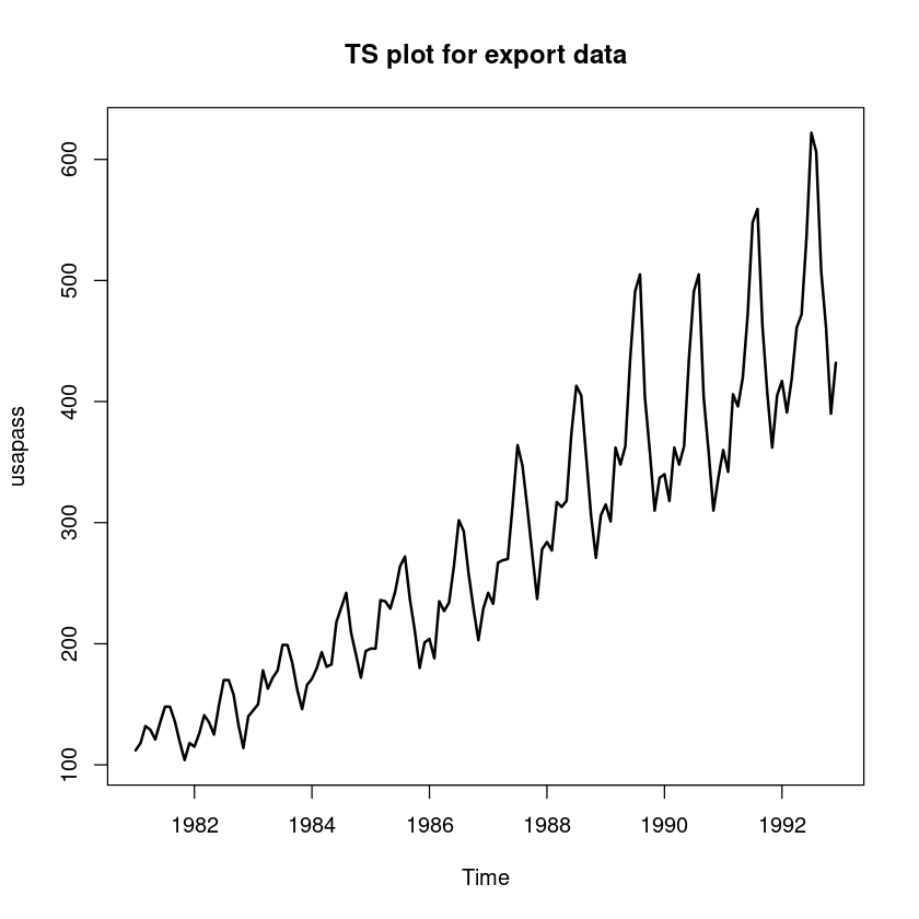

usapass_l <- ts(log(z5), start=c(1981,1), frequency=12)
plot.ts(usapass_l, lwd=2, main="TS plot for export data")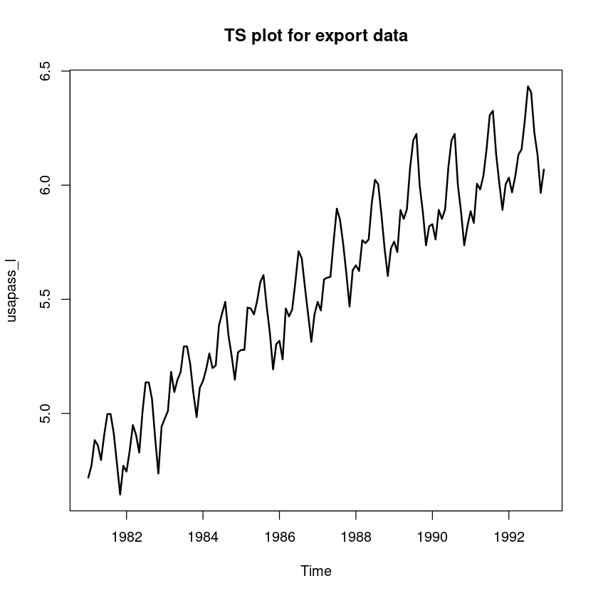

(1)

왜 log 변환이 필요한지에 대해 간단히 설명하여라.

시도표를 확인하면 시간에 따라 분산이 커지는 것을 볼수 있다. 이는 모델의 결과가 잘못된 값이 나올 수 있다.

(2)

적절한 추세 모형을 적합시킨 후 잔차분석을 하여라.

z5_ts <- ts(z5, frequency=12)
cycle(z5_ts)

A Time Series: 12 × 12

	Jan	Feb	Mar	Apr	May	Jun	Jul	Aug	Sep	Oct	Nov	Dec
1	1	2	3	4	5	6	7	8	9	10	11	12
2	1	2	3	4	5	6	7	8	9	10	11	12
3	1	2	3	4	5	6	7	8	9	10	11	12
4	1	2	3	4	5	6	7	8	9	10	11	12
5	1	2	3	4	5	6	7	8	9	10	11	12
6	1	2	3	4	5	6	7	8	9	10	11	12
7	1	2	3	4	5	6	7	8	9	10	11	12
8	1	2	3	4	5	6	7	8	9	10	11	12
9	1	2	3	4	5	6	7	8	9	10	11	12
10	1	2	3	4	5	6	7	8	9	10	11	12
11	1	2	3	4	5	6	7	8	9	10	11	12
12	1	2	3	4	5	6	7	8	9	10	11	12

seasonal_I <- as.factor(cycle(z5_ts))
t <- 1:length(z5)
m3 <- lm(log(z5)~t+seasonal_I)

summary(m3)

Call:
lm(formula = log(z5) ~ t + seasonal_I)

Residuals:
      Min        1Q    Median        3Q       Max 
-0.159814 -0.044426  0.000623  0.045572  0.151846 

Coefficients:
               Estimate Std. Error t value Pr(>|t|)    
(Intercept)   4.7246982  0.0198289 238.274  < 2e-16 ***
t             0.0100999  0.0001252  80.666  < 2e-16 ***
seasonal_I2  -0.0220859  0.0254094  -0.869  0.38633    
seasonal_I3   0.1095029  0.0254104   4.309 3.19e-05 ***
seasonal_I4   0.0768102  0.0254119   3.023  0.00302 ** 
seasonal_I5   0.0762636  0.0254141   3.001  0.00322 ** 
seasonal_I6   0.1990500  0.0254168   7.831 1.45e-12 ***
seasonal_I7   0.3049668  0.0254202  11.997  < 2e-16 ***
seasonal_I8   0.2976260  0.0254242  11.706  < 2e-16 ***
seasonal_I9   0.1461189  0.0254289   5.746 6.08e-08 ***
seasonal_I10  0.0110851  0.0254341   0.436  0.66367    
seasonal_I11 -0.1341418  0.0254399  -5.273 5.39e-07 ***
seasonal_I12 -0.0214153  0.0254464  -0.842  0.40156    
---
Signif. codes:  0 ‘***’ 0.001 ‘**’ 0.01 ‘*’ 0.05 ‘.’ 0.1 ‘ ’ 1

Residual standard error: 0.06224 on 131 degrees of freedom
Multiple R-squared:  0.982, Adjusted R-squared:  0.9803 
F-statistic: 594.1 on 12 and 131 DF,  p-value: < 2.2e-16

• 적합된 모형: \(\hat Z_t = 4.72 + 0.01t - 0.022I_{t2} + \dots - 0.021 I_{t12}\)

tmp.data <- data.frame(
 day = seq(ymd("1984-01-01"),
 by='1 month', length.out=length(z5)),
 z=z5
)

par(mfrow=c(2,1)) 
plot(z~day, tmp.data, type='l')
lines(tmp.data$day, exp(fitted(m3)), col='red', lty=2, lwd=2)    # m3에 exp함수 처리
plot(log(z)~day, tmp.data, type='l')
lines(tmp.data$day, fitted(m3), col='red', lty=2, lwd=2)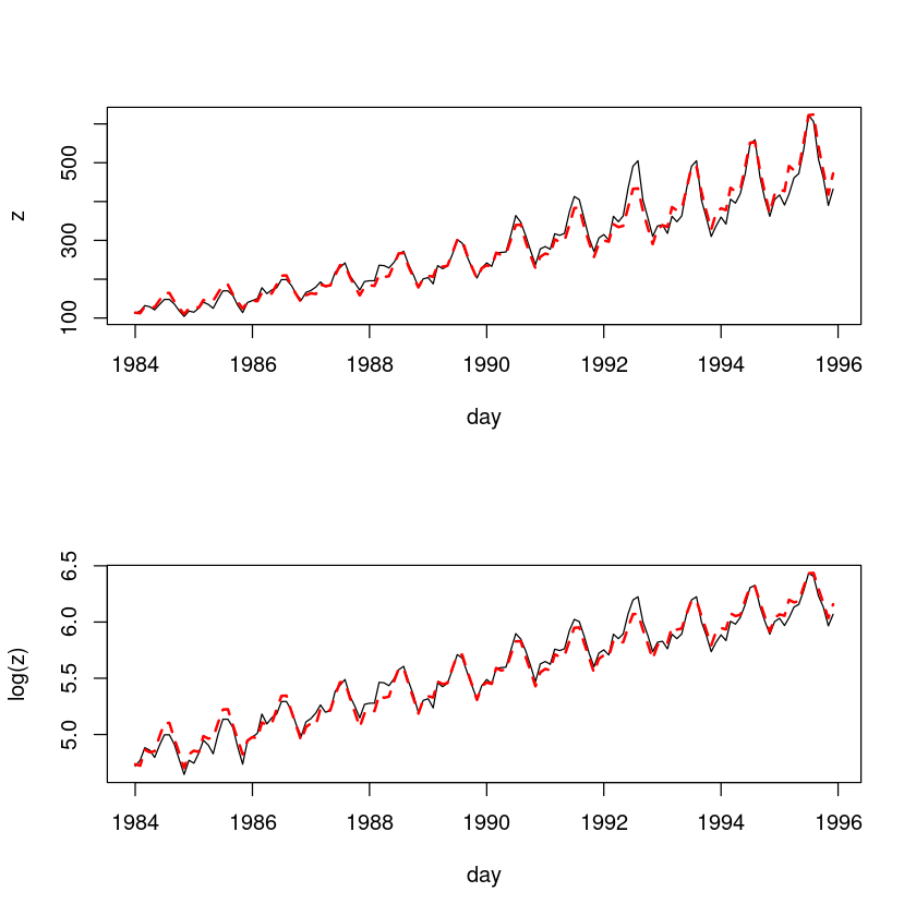

resid_m3 <- resid(m3)
plot(resid_m3, pch=16, type='l')
abline(h=0, lty=2)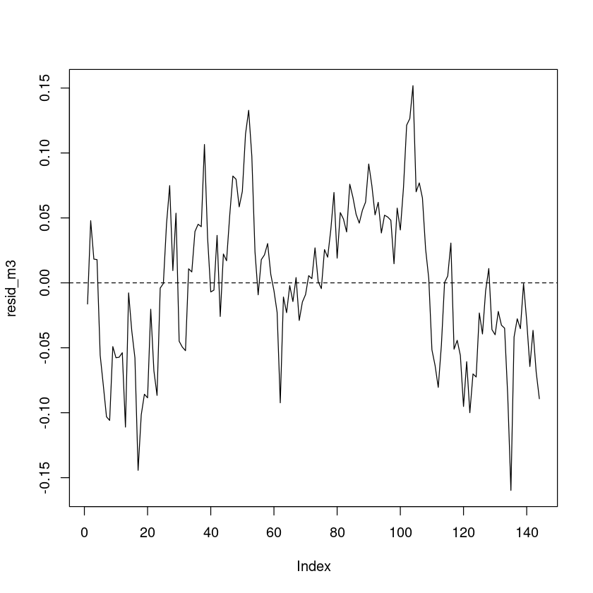

t.test(resid_m3)

    One Sample t-test

data:  resid_m3
t = 1.4082e-16, df = 143, p-value = 1
alternative hypothesis: true mean is not equal to 0
95 percent confidence interval:
 -0.009812747  0.009812747
sample estimates:
   mean of x 
6.990845e-19 

hist(resid_m3)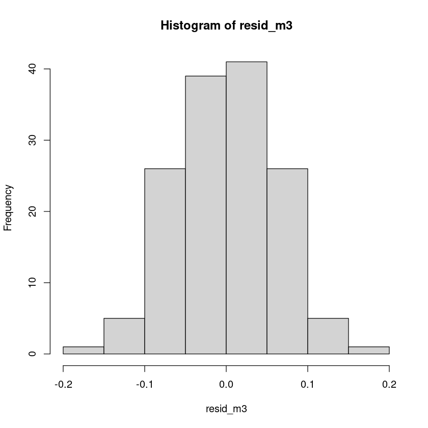

lmtest::bptest(m3)

    studentized Breusch-Pagan test

data:  m3
BP = 5.9163, df = 12, p-value = 0.9202

lmtest::dwtest(m3, alternative="two.sided")

    Durbin-Watson test

data:  m3
DW = 0.40831, p-value < 2.2e-16
alternative hypothesis: true autocorrelation is not 0

sum((summary(m3)$residual)^2)

0.507459833285849

(3)

적절한 평활법을 적용한 후 잔차분석을 하여라.

가법모형

fit_hw_l <- HoltWinters(usapass_l, seasonal="additive")

fit_hw_l

Holt-Winters exponential smoothing with trend and additive seasonal component.

Call:
HoltWinters(x = usapass_l, seasonal = "additive")

Smoothing parameters:
 alpha: 0.3447498
 beta : 0.003585913
 gamma: 0.879488

Coefficients:
            [,1]
a    6.165298459
b    0.008744433
s1  -0.073696849
s2  -0.142822821
s3  -0.039964334
s4   0.015968620
s5   0.033673237
s6   0.157016140
s7   0.300626468
s8   0.285698068
s9   0.098491289
s10 -0.021898771
s11 -0.190036243
s12 -0.096734648

par(mfrow=c(2,1)) 
plot(z~day, tmp.data, type='l')
lines(tmp.data$day, exp(fitted(m3)), col='red', lty=2, lwd=2)    # m3에 exp함수 처리
plot(log(z)~day, tmp.data, type='l')
lines(tmp.data$day, fitted(m3), col='red', lty=2, lwd=2)

fit6= hw(usapass_l,
 alpha = fit_hw_l$alpha,
 beta = fit_hw_l$beta,
 gamma = fit_hw_l$gamma,
 seasonal="additive",
 initial="simple",
 h=12)
fit6$model

Holt-Winters' additive method 

Call:
 hw(y = usapass_l, h = 12, seasonal = "additive", initial = "simple",  

 Call:
     alpha = fit_hw_l$alpha, beta = fit_hw_l$beta, gamma = fit_hw_l$gamma) 

  Smoothing parameters:
    alpha = 0.3447 
    beta  = 0.0036 
    gamma = 0.8795 

  Initial states:
    l = 4.8362 
    b = 0.0079 
    s = -0.0655 -0.1918 -0.0571 0.0765 0.161 0.161
           0.0691 -0.0404 0.0236 0.0466 -0.0655 -0.1177

  sigma:  0.0425

- 원데이터와 비교그림 넣어주기 위해서 exp취해줌

plot(usapass)
lines(exp(fit6$fitted), lwd=3, col='red', lty=2)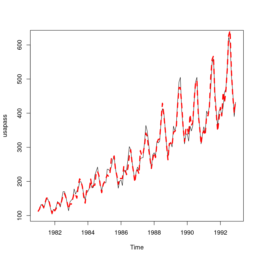

ts.plot(fit6$residual, ylab="residual",
 main="가법모형의 잔차 그림"); abline(h=0)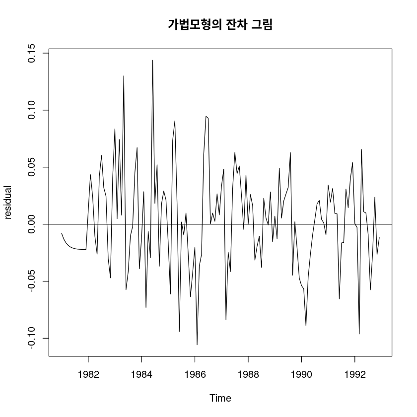

t.test(fit6$residual)

    One Sample t-test

data:  fit6$residual
t = 0.72402, df = 143, p-value = 0.4702
alternative hypothesis: true mean is not equal to 0
95 percent confidence interval:
 -0.004441394  0.009575433
sample estimates:
  mean of x 
0.002567019 

dwtest(lm(fit6$residual~1), alternative = 'two.sided')

    Durbin-Watson test

data:  lm(fit6$residual ~ 1)
DW = 1.5421, p-value = 0.005659
alternative hypothesis: true autocorrelation is not 0

승법모형(원데이터로 진행해봄)

fit_hw_m <- HoltWinters(usapass, seasonal="multiplicative")

plot(fit_hw_m)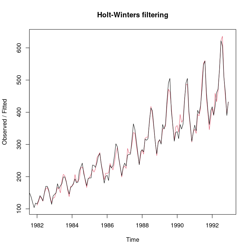

fit7= hw(usapass,
 alpha = fit_hw_m$alpha,
 beta = fit_hw_m$beta,
 gamma = fit_hw_m$gamma,
 seasonal="multiplicative",
 initial="simple",
 h=12)
fit7$model

Holt-Winters' multiplicative method 

Call:
 hw(y = usapass, h = 12, seasonal = "multiplicative", initial = "simple",  

 Call:
     alpha = fit_hw_m$alpha, beta = fit_hw_m$beta, gamma = fit_hw_m$gamma) 

  Smoothing parameters:
    alpha = 0.3205 
    beta  = 0.0239 
    gamma = 1 

  Initial states:
    l = 126.6667 
    b = 1.0833 
    s = 0.9316 0.8211 0.9395 1.0737 1.1684 1.1684
           1.0658 0.9553 1.0184 1.0421 0.9316 0.8842

  sigma:  0.0465

ts.plot(fit7$residual, ylab="residual",
 main="승법모형의 잔차 그림"); abline(h=0)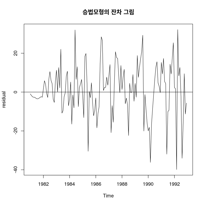

t.test(fit7$residual)

    One Sample t-test

data:  fit7$residual
t = 1.0873, df = 143, p-value = 0.2787
alternative hypothesis: true mean is not equal to 0
95 percent confidence interval:
 -0.9675137  3.3332414
sample estimates:
mean of x 
 1.182864 

dwtest(lm(fit7$residual~1), alternative = 'two.sided')

    Durbin-Watson test

data:  lm(fit7$residual ~ 1)
DW = 1.4311, p-value = 0.0005873
alternative hypothesis: true autocorrelation is not 0

(4)

적절한 분해법에 의해 각 성분을 분해해여 시계열 그림을 그려라.

decopose분해법

dec_f_a_l <- decompose(usapass_l, 'additive')

plot(dec_f_a_l) # 로그변환 후 분해법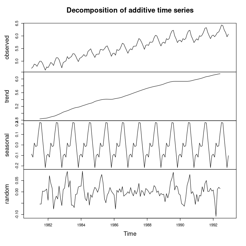

# ## 승법모형 비교용
# dec_f_m <- decompose(usapass, type = "multiplicative")
# plot(dec_f_m)

pred_dec_ <- dec_f_a_l$trend + dec_f_a_l$seasonal

## 가법모형 vs. 승법모형
pred_dec_ <-dec_f_a_l$trend+dec_f_a_l$seasonal
pred_dec2_ <-dec_f_m$trend*dec_f_m$seasonal

ts.plot(exp(pred_dec_), pred_dec2_, col=1:2, lty=1:2, ylab="usapass", xlab="time")
legend("topleft", lty=1:2, col=1:2, c("가법모형", "승법모형"))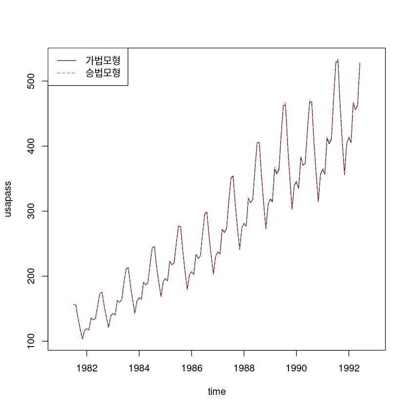

sum((usapass_l-pred_dec_)^2, na.rm=T) 

0.161507492507272

stl(비교용)

stl_fit11 <- stl(usapass_l, s.window=12)

plot(stl_fit11)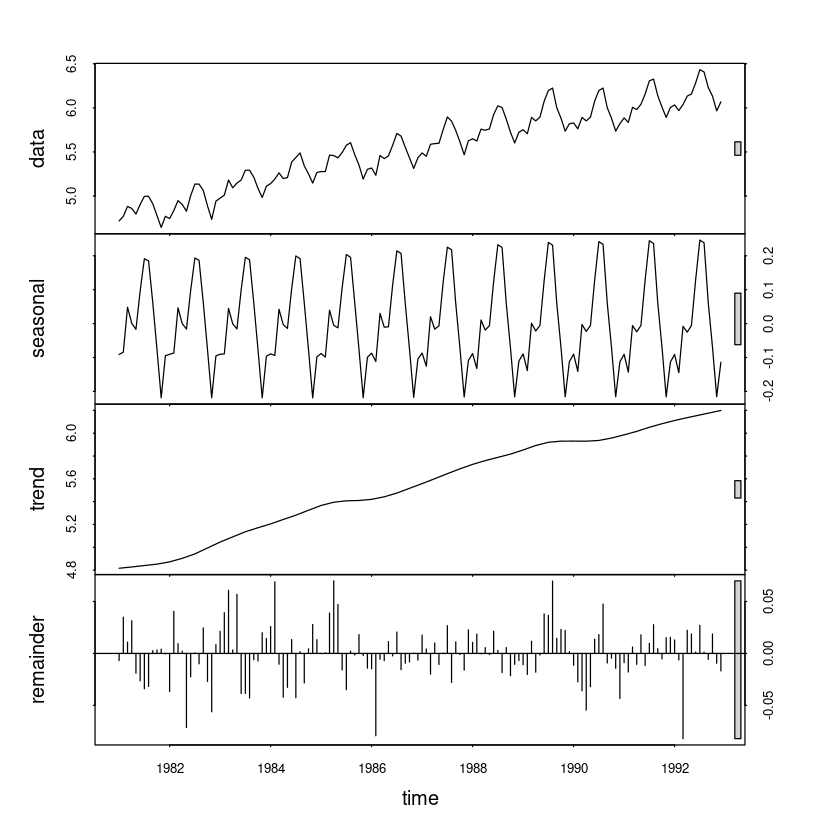

## stl vs. decompose
pred_stl <- stl_fit11$time.series[,1]+stl_fit11$time.series[,2]

ts.plot(pred_stl, pred_dec_, col=1:2, lty=1:2, lwd=2:3, ylab="food", xlab="time",
     main="stl vs. decomse")
legend("topleft", lty=1:2, col=1:2, c("stl", "decomse"))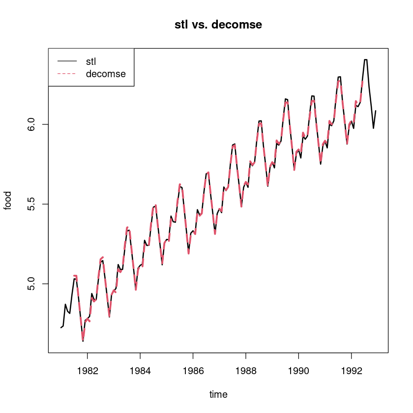

### SSE : 1-시차 후 예측 오차 제곱합
sum((usapass_l-pred_stl)^2) #144
sum((usapass_l-pred_dec_)^2, na.rm=T) #144-12=132

0.101745211385709

0.161507492507272

추세를 이용한 분해법(가법)

fit45 <- lm(usapass_l ~ t)
summary(fit45)

Call:
lm(formula = usapass_l ~ t)

Residuals:
     Min       1Q   Median       3Q      Max 
-0.30875 -0.10481 -0.01736  0.09677  0.36311 

Coefficients:
             Estimate Std. Error t value Pr(>|t|)    
(Intercept) 4.8131072  0.0237011  203.07   <2e-16 ***
t           0.0100802  0.0002836   35.54   <2e-16 ***
---
Signif. codes:  0 ‘***’ 0.001 ‘**’ 0.01 ‘*’ 0.05 ‘.’ 0.1 ‘ ’ 1

Residual standard error: 0.1415 on 142 degrees of freedom
Multiple R-squared:  0.899, Adjusted R-squared:  0.8982 
F-statistic:  1263 on 1 and 142 DF,  p-value: < 2.2e-16

• \(\hat T_t = 4.8131072 + 0.0100802t\)

hat_Tt_l <- fitted(fit45)

ts.plot(usapass_l, hat_Tt_l,
     col=1:2,
     lty=1:2,
     lwd=2:3,
     ylab="usapass_l", xlab="time",
     main="log변환한 시계열과 분해법에 의한 추세성분")
legend("topleft", lty=1:2, col=1:2, lwd=2:3, c("ln(z)", "추세성분"))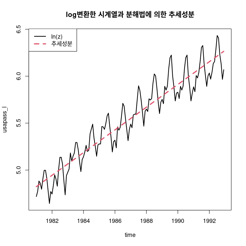

## 원시계열에서 추세성분 조정
adjtrend_l = usapass_l-hat_Tt_l
plot.ts(adjtrend_l, lwd=2)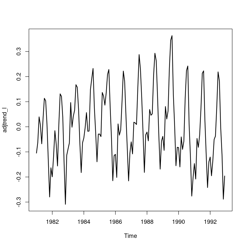

## 지시함수를 이용한 계절성분 추정
y = factor(cycle(adjtrend_l)) #범주형 변수로 변환

fit456 <- lm(adjtrend_l ~ 0+y)
summary(fit456)

Call:
lm(formula = adjtrend_l ~ 0 + y)

Residuals:
      Min        1Q    Median        3Q       Max 
-0.158515 -0.044012  0.001096  0.045041  0.152437 

Coefficients:
    Estimate Std. Error t value Pr(>|t|)    
y1  -0.08709    0.01790  -4.865 3.20e-06 ***
y2  -0.10916    0.01790  -6.098 1.11e-08 ***
y3   0.02245    0.01790   1.254  0.21195    
y4  -0.01022    0.01790  -0.571  0.56899    
y5  -0.01075    0.01790  -0.600  0.54926    
y6   0.11206    0.01790   6.260 5.00e-09 ***
y7   0.21799    0.01790  12.178  < 2e-16 ***
y8   0.21067    0.01790  11.769  < 2e-16 ***
y9   0.05919    0.01790   3.306  0.00122 ** 
y10 -0.07583    0.01790  -4.236 4.24e-05 ***
y11 -0.22103    0.01790 -12.348  < 2e-16 ***
y12 -0.10829    0.01790  -6.049 1.40e-08 ***
---
Signif. codes:  0 ‘***’ 0.001 ‘**’ 0.01 ‘*’ 0.05 ‘.’ 0.1 ‘ ’ 1

Residual standard error: 0.06201 on 132 degrees of freedom
Multiple R-squared:  0.8214,    Adjusted R-squared:  0.8052 
F-statistic: 50.59 on 12 and 132 DF,  p-value: < 2.2e-16

\(\hat S_t = -0.08709I_1 + \dots - 0.10829I_{12}\)

hat_St_l <- fitted(fit456)
ts.plot(hat_St_l, main="추정된 계절성분")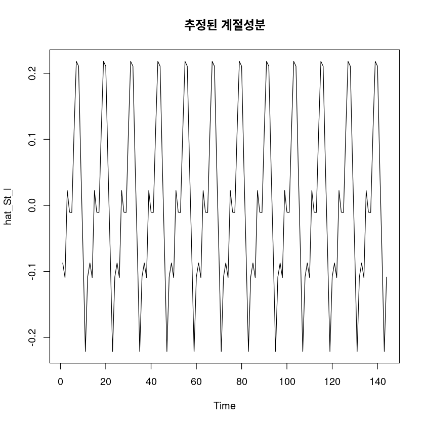

hat_It_l <- usapass_l - hat_Tt_l - hat_St_l
ts.plot(hat_It_l); abline(h=0)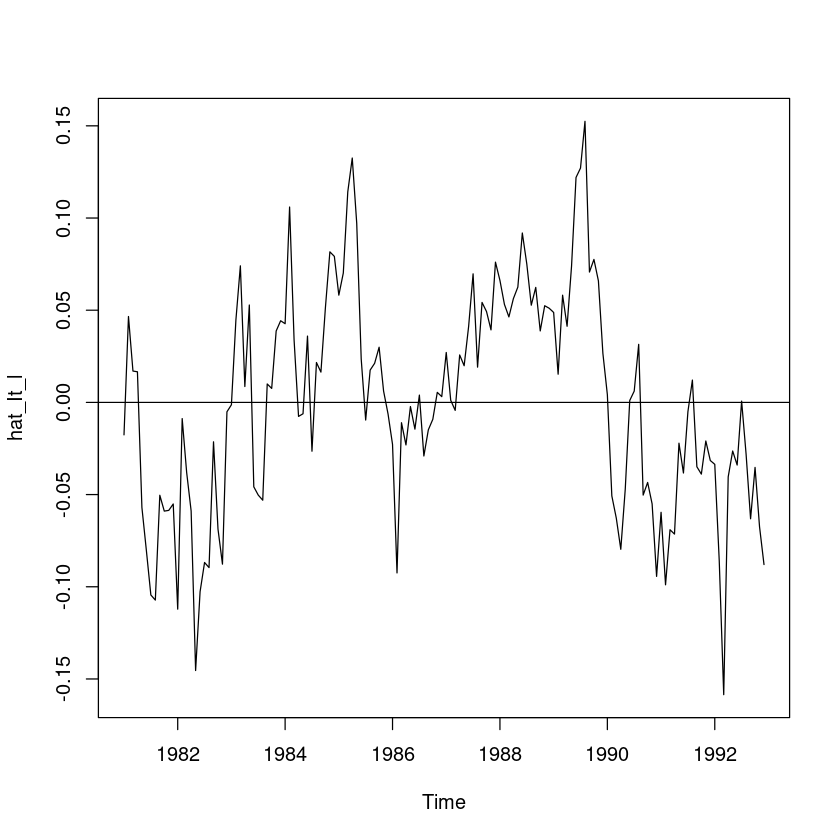

- 추정

pred_a_l <- hat_Tt_l + hat_St_l

ts.plot(usapass, exp(pred_a_l), col=1:2, lty=1:2, lwd=2:3,ylab="usapass", xlab="time",
     main="시계열과 분해법에 의한 추정값")
legend("topleft", lty=1:2, col=1:2, c("Z", "추정값"))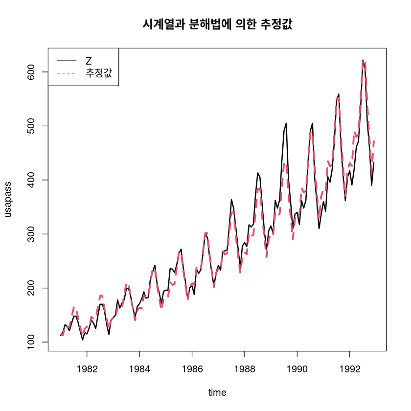

추세를 이용한 분해법(승법)

## 추세성분 추정
fit5 <- lm(usapass ~ t ) 
summary(fit5)

Call:
lm(formula = usapass ~ t)

Residuals:
    Min      1Q  Median      3Q     Max 
-95.238 -31.381  -6.677  24.113 163.347 

Coefficients:
            Estimate Std. Error t value Pr(>|t|)    
(Intercept) 87.41968    7.91971   11.04   <2e-16 ***
t            2.67074    0.09477   28.18   <2e-16 ***
---
Signif. codes:  0 ‘***’ 0.001 ‘**’ 0.01 ‘*’ 0.05 ‘.’ 0.1 ‘ ’ 1

Residual standard error: 47.27 on 142 degrees of freedom
Multiple R-squared:  0.8483,    Adjusted R-squared:  0.8473 
F-statistic: 794.3 on 1 and 142 DF,  p-value: < 2.2e-16

• \(\hat T_t = 87.41968 + 2.67074t\)

ts.plot(usapass, fitted(fit5) , col=1:2, lty=1:2, lwd=2:3, ylab="usapass", xlab="time",
 main="원시계열과 분해법에 의한 추세성분")
legend("topleft", lty=1:2, col=1:2, c("원시계열", "추세성분"))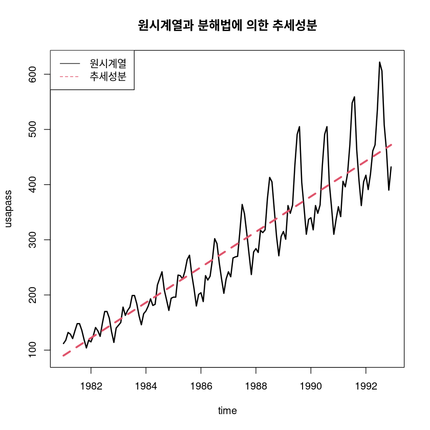

fit5_ <- lm(usapass ~ t + I(t^2)) 
summary(fit5_)

Call:
lm(formula = usapass ~ t + I(t^2))

Residuals:
     Min       1Q   Median       3Q      Max 
-101.286  -27.201   -7.821   20.791  145.107 

Coefficients:
             Estimate Std. Error t value Pr(>|t|)    
(Intercept) 1.113e+02  1.172e+01   9.494  < 2e-16 ***
t           1.689e+00  3.733e-01   4.525 1.27e-05 ***
I(t^2)      6.770e-03  2.494e-03   2.715  0.00746 ** 
---
Signif. codes:  0 ‘***’ 0.001 ‘**’ 0.01 ‘*’ 0.05 ‘.’ 0.1 ‘ ’ 1

Residual standard error: 46.25 on 141 degrees of freedom
Multiple R-squared:  0.8559,    Adjusted R-squared:  0.8538 
F-statistic: 418.6 on 2 and 141 DF,  p-value: < 2.2e-16

ts.plot(usapass, fitted(fit5), fitted(fit5_), col=1:3, lty=1:2, lwd=2:3, ylab="usapass",
 main="원시계열과 분해법에 의한 추세성분")
legend("topleft", lty=1:2, col=1:3, c("원시계열", "추세성분", "2차 추세성분"))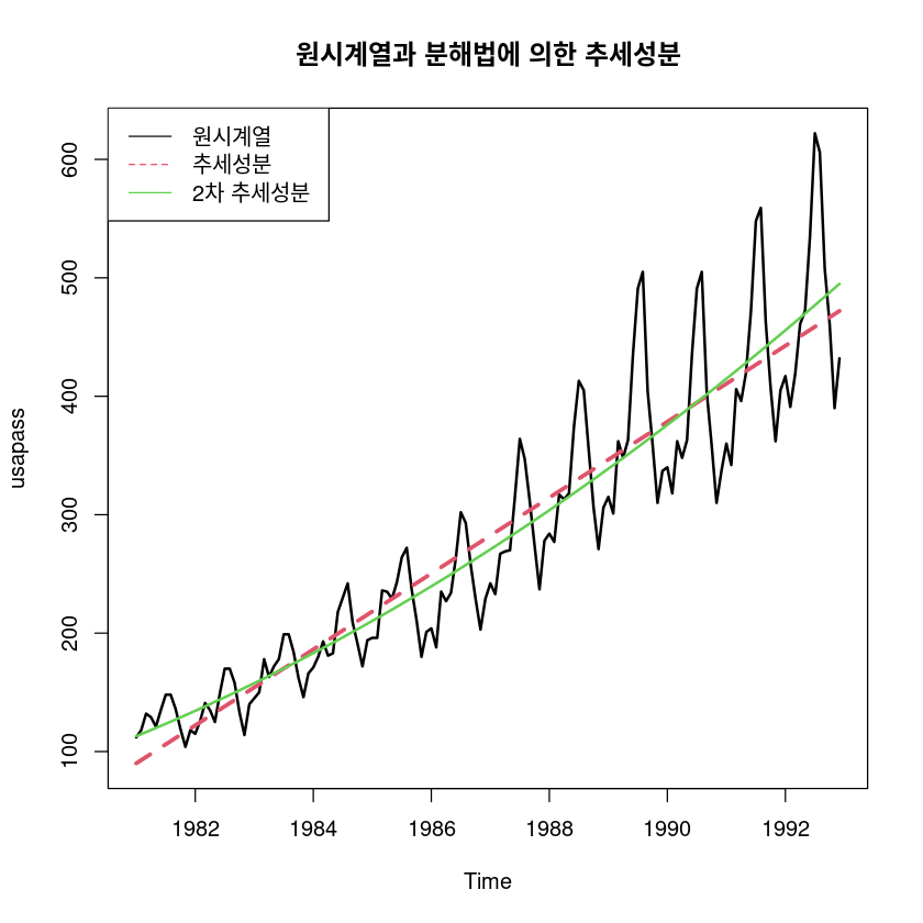

## 원시계열에서 추세성분 조정
trend_5 = fitted(fit5)  # 1차 추세모형
adjtrend_5 = usapass/trend_5
plot.ts(adjtrend_5)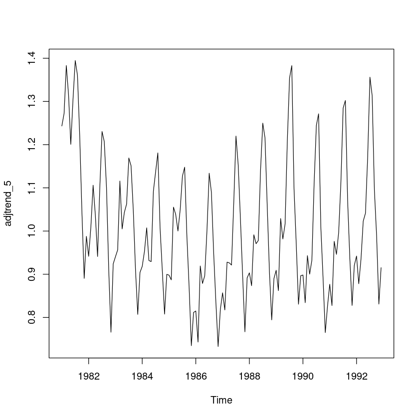

## 원시계열에서 2차 추세성분 조정
trend_5_ = fitted(fit5_)  # 2차 추세모형
adjtrend_5_ = usapass/trend_5_
plot.ts(adjtrend_5_)
abline(h=1, lty=2)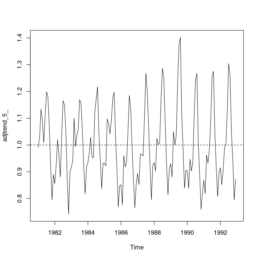

## 지시함수를 이용한 계절성분 추정
y = factor(cycle(adjtrend_5_)) 
fit55 <- lm(adjtrend_5_ ~ 0+y)
summary(fit55)

Call:
lm(formula = adjtrend_5_ ~ 0 + y)

Residuals:
      Min        1Q    Median        3Q       Max 
-0.115502 -0.040795  0.001315  0.026514  0.177535 

Coefficients:
    Estimate Std. Error t value Pr(>|t|)    
y1   0.91079    0.01538   59.22   <2e-16 ***
y2   0.89219    0.01538   58.01   <2e-16 ***
y3   1.01655    0.01538   66.10   <2e-16 ***
y4   0.98286    0.01538   63.91   <2e-16 ***
y5   0.98163    0.01538   63.83   <2e-16 ***
y6   1.10939    0.01538   72.13   <2e-16 ***
y7   1.23340    0.01538   80.20   <2e-16 ***
y8   1.22448    0.01538   79.62   <2e-16 ***
y9   1.05099    0.01538   68.34   <2e-16 ***
y10  0.91823    0.01538   59.70   <2e-16 ***
y11  0.79424    0.01538   51.64   <2e-16 ***
y12  0.88904    0.01538   57.81   <2e-16 ***
---
Signif. codes:  0 ‘***’ 0.001 ‘**’ 0.01 ‘*’ 0.05 ‘.’ 0.1 ‘ ’ 1

Residual standard error: 0.05328 on 132 degrees of freedom
Multiple R-squared:  0.9974,    Adjusted R-squared:  0.9972 
F-statistic:  4301 on 12 and 132 DF,  p-value: < 2.2e-16

\(\hat S_t = 0.91079I_1 + \dots + 0.88904I_{12}\)

seasonal <- fitted(fit55)
ts.plot(seasonal, main="추정된 계절성분")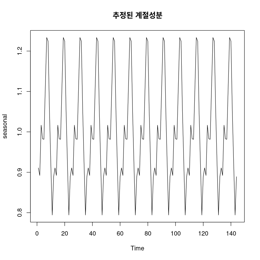

ts.plot(adjtrend_5_, seasonal, col=1:2, lty=1:2, lwd=2:3, main="추세조정된 시계열")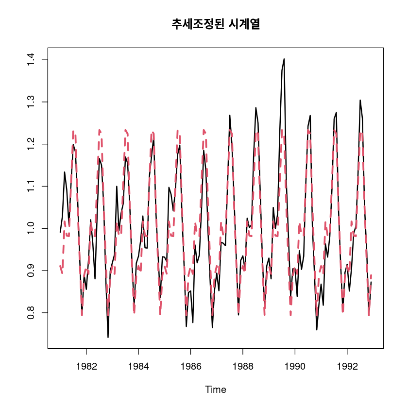

irregular5 <- usapass/trend_5/seasonal

ts.plot(irregular5); abline(h=1, lty=2)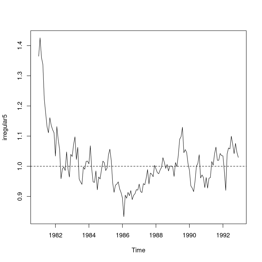

t.test(irregular5, mu=1)

    One Sample t-test

data:  irregular5
t = 1.2411, df = 143, p-value = 0.2166
alternative hypothesis: true mean is not equal to 1
95 percent confidence interval:
 0.994507 1.024030
sample estimates:
mean of x 
 1.009268 

dwtest(lm(irregular5~ 1), alternative = 'two.sided')

    Durbin-Watson test

data:  lm(irregular5 ~ 1)
DW = 0.19413, p-value < 2.2e-16
alternative hypothesis: true autocorrelation is not 0

pred_m5 <- trend_5 * seasonal

ts.plot(usapass, pred_m5, col=1:2, lty=1:2, lwd=2:3, ylab="food", xlab="time",
 main="원시계열과 분해법에 의한 추정값")
legend("topleft", lty=1:2, col=1:2, c("원시계열", "추정값"))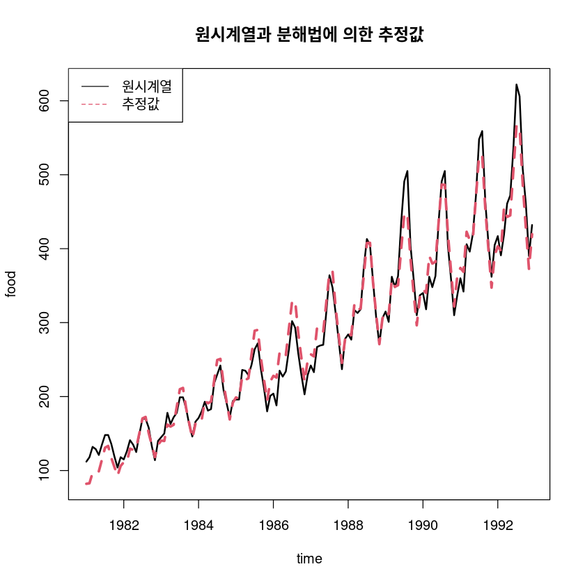

(5) 틀림 ㅠㅠ

각 분석방법에 의한 결과를 1-시착 후 예측오차의 제곱합 (SSE) 기준하에서 비교하여라.

- 추세모형

sum((m3$residuals)^2)

0.507459833285849

- 평활법

exp(fit_hw_l$SSE)

1.24913252727246

- decompose

sum((usapass_l-pred_dec_)^2, na.rm=T) #SSE - 가법

0.161507492507272

- stl

sum((usapass_l-pred_stl)^2,na.rm=T)

0.101745211385709

- 추세를 이용한 분해법(가법)

sum((usapass_l-pred_a_l)^2)

0.507555612028427